Modern hard drives store an incredible amount of data in a small space, and are still the default choice for high-capacity (though not highest-performance) storage. While hard drives have been around since the 1950s, the current 3.5″ form factor (actually 4″ wide) appeared in the early 1980s. Since then, the capacity of a 3.5″ drive has increased by about 106 times (from 10 MB to about 10 TB), sequential throughput by about 103 times, and access times by about 101 times. Although the basic concept of spinning magnetic disks accessed by a movable stack of disk heads has not changed, hard drives have become much more complex to enable the increased density and performance. Early drives had tens of thousands of sectors arranged in hundreds of concentric tracks (sparse enough for a stepper motor to accurately position the disk head), while current drives have billions of sectors (with thousands of defects), packed into hundreds of thousands of tracks spaced tens of nanometers apart.
Beyond just the high-level performance (throughput and seek time) measurements, which drive characteristics can be characterized using microbenchmarks? I had initially set out to detect the number of platters in a disk without opening up a disk, but in modern disks this simple-sounding task requires measuring several other properties before inferring the count of recording surfaces. Characterizing disk drive geometry has been done in the past [1, 2], and the algorithms I used aren’t very different. However, older algorithms often make assumptions that are no longer true on modern drives. For example, the Skippy [2] algorithm (a fast algorithm to measure the number of surfaces, cylinder switch times, and head switch times) no longer works on modern drives because the algorithm assumes one particular ordering of tracks onto multiple platters that is no longer used on modern disks (that several head switches occur before a seek to the next cylinder).
Hard disk drives store data on a stack of one or more rotating magnetic disks. Data is written in concentric tracks. A stack of read/write heads move (radially) across the disks to position the head over the desired track. There are typically two heads per platter (one for each side), and the entire stack of heads move together as a single unit. Reading data occurs by moving the disk head to the desired track (a seek), waiting until the beginning of the desired data passes under the disk head, and then continuing to read sequentially until either all of the requested data is read, or the end of the track, when the head needs to be moved to the next track. A hard drive’s “geometry” describes how data is arranged into platters, tracks, and sectors. Historically, this was described using three numbers: Cylinders (number of concentric rings from outside to inside), Heads (number of recording surfaces, or the number of tracks per cylinder), and Sectors per track, leading to the well-known acronym CHS. The capacity of a hard drive in sectors is simply C×H×S. Today, C and S are variable and only H is still constant. The number of tracks is not necessarily the same on each recording surface, and the number of sectors per track varies across the disk (more sectors in the longer outer tracks than the inner tracks).
This article describes several microbenchmarks that try to extract the physical geometry of hard disk drives, and a few other related measurements. These measurements include rotation period, the physical location (angle and radius) of each sector, track boundaries, skew, seek time, and some observations of defective sectors. I use these microbenchmarks to characterize a variety of hard drives from 45 MB (1989) to 5 TB (2015). There is no attempt to characterize other important performance aspects such as caching. The remainder of this article begins with a background on hard drive geometry. It then describes the collection of microbenchmarks, starting with a basic read access time measurement and building towards increasingly complex algorithms. The second part of the article presents microbenchmark measurements for each of the 17 drives that were tested.
Summary
- Background: Hard drives consist of spinning disks, and a stack of heads. Data is arranged on recording surfaces (2 sides per platter), tracks, and sectors. “Cylinders” no longer exist in drives newer than around 2000.
- What can be measured: RPM, angular position of every sector, and seek times, by timing specific sequences of sector reads. These basic measurement methods can then be used to find track boundaries, how tracks are arranged on a surface, and the number of surfaces.
- Access time: Out of the drives I tested, it takes 1.3 to 3.6 revolutions to do a full-stroke seek.
- Heads accelerate slowly: Very few tracks are accessible in the first revolution.
- Short stroking offers limited reduction in seek times because even short seeks take a relatively long time.
- Seek time is non-trivial to measure.
- A seek time plot can be used to observe acoustic management (AAM). AAM slows down long-distance seeks to reduce noise, but not short-distance seeks.
- Track boundaries can be found by searching the disk for track skew. Newer disks use different densities (track size) on each surface.
- Track density and bit density can be estimated by knowing track count and size. In the newest drive I have, average track pitch is 80 nm and an average bit is 17 nm in length.
- Combining seek profile and track size together usually reveals the track layout.
- There is a large diversity of track layouts. Old drives had “cylinders” (several head switches occurs before a seek to the next track), but new drives use groups of adjacent tracks before changing heads.
- Track skew can be measured using track boundary information.
- There is more than one type of skew. A cylinder, serpentine, or zone change usually uses a bigger skew than for adjacent tracks.
- Track skew is usually constant from beginning to end of the drive, but not on the Maxtor 7405AV. Track skew is usually the same on every recording surface, but not on the Seagate ST1.
- Combining the above tools can find and visualize defective sectors. Most disks have holes of defective sectors, while some skip over entire tracks.
- Microbenchmarking is hard. Despite much effort, my algorithms do not work flawlessly.
- Measurement results for 17 hard drive models from 45 MB to 5 TB on Page 2.
Background: Hard drive geometry

Sectors, tracks, and cylinders. A cylinder is the collection of all tracks at the same radius (6 tracks per cylinder shown here, on two sides and three platters).
As seen by software, a hard drive looks like a big block of sectors, traditionally 512 bytes each (now 4,096 bytes), with little knowledge of the physical location of the sectors. For example, a 300 GB drive might have 585,937,500 512-byte sectors, numbered 0 through 585,937,499. Some early hard drive interfaces required the drive controller on the host computer to know the physical layout of the disk (because the controller sent commands to move the disk head). IDE hard drives (Integrated Drive Electronics, mid 1980s) finally integrated the disk controller into the drive. The integrated disk controller translates logical (as seen by software) sector numbers into physical locations, which presents a simple block-of-sectors interface to the host computer while allowing much more complex physical layouts. Unfortunately, for software compatibility reasons, the sector number was still encoded as a CHS triplet (three numbers, but unrelated to the true number of cylinders, heads, or sectors/track of the drive) for many more years until LBA (logical block addressing, encoding a sector number as one number) became popular.
While logically just a big block of sectors, sectors, tracks, and heads (or recording surfaces) still physically exist. There is just no easy way for software to know about them. This section gives some basic definitions for these physical features. Many readers may already be familiar with these.
Sector
Data is stored in blocks of equal size. A sector is the smallest unit of data that can be read or written to a disk. 512-byte sectors have been standard since the 1980s, while new drives (around 2011) use 4096-byte sectors (branded as Advanced Format).
Sectors have additional metadata that are also written to the disk surface (such as its sector number and error correction codes). On drives using embedded servo (all non-ancient drives), there are also servo patterns on the disk which are used to position the disk head. All of this occupies space on the disk surface but is invisible to the host.
Tracks
A track is a circle of consecutive sectors placed on one disk surface along one revolution of the disk. Reading sectors within a track is done by having the head follow the track while the disk rotates. Crossing a track boundary requires moving the disk head to the next track (a track-to-track seek) or switching to a different head to read a track from a different disk surface (a head switch). Prior to zone bit recording, every track on a disk was the same size (number of sectors). Zone bit recording packs more sectors into physically-longer outside tracks and fewer in the shorter inner tracks. Because one track (regardless of length) is read per revolution, hard drives have higher throughput near the beginning of the drive. Track size can also vary between recording surfaces, because the recording surface and head quality varies even within a single drive.
Hard drives (like floppy disks) use concentric circular tracks, unlike CDs and DVDs which use a single spiral track.
Cylinders
A cylinder is a collection of tracks on multiple surfaces that are located at the same radius (If a track is a circle, then a stack of circles of the same diameter forms a cylinder). On older drives, tracks on different surfaces were aligned so that accessing tracks within the same cylinder only required switching heads (a faster electrical operation) but not moving the heads (a slower mechanical operation). Cylinders are no longer meaningful on modern drives. With increased track density, tracks on different recording surfaces aren’t aligned well enough to form cylinders and a head switch requires a larger head movement than moving to an adjacent track on the same surface, which makes a head switch slower than moving to an adjacent track.
Zones
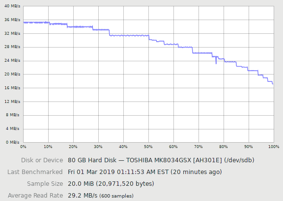
Disk throughput benchmark. About 20 zones are visible. Outer tracks have higher throughput than inner tracks, and throughput is constant within a zone.
Because the outer tracks are physically longer, more sectors can be packed into outer tracks than the inner tracks. For simplicity, adjacent tracks are grouped into zones where every track within a zone has the same track size (number of sectors per track). Zone bit recording gives the familiar throughput curve where outer tracks have higher throughput than inner tracks, with throughput decreasing in discrete steps.
Traditionally, zones were thought of as groups of cylinders, where all tracks on all surfaces in the zone had the same size. Because track size on modern drives can differ between recording surfaces, it only makes sense to think of a zone as a group of adjacent tracks on the same recording surface on modern drives.
Track Skew
Left: No skew. Every track starts at the same angular position. There is one wasted revolution after every track because it takes non-zero time to move to the next track. Right: Skew of 72° (1/5 revolution). After finishing a track, only 1/5 of a revolution is wasted if the head can move to the next track within that time.
Sequential accesses read a track over one complete revolution, moves the head to the next track, then reads for another revolution. If all tracks started at the same angular position, the non-zero time to move to the next track would cause the head to miss the beginning of the next track by the time the head arrives, causing almost one complete revolution to be wasted. To mitigate this, each track is skewed so that it starts somewhat later than the previous track to give the disk head enough time to move from the end of the previous track to the start of the next track before the first sector of the next track appears under the head. With a proper choice of track skew, only a fraction of a rotation is wasted in between tracks. The drives I tested had skews from 6% to 36% of a rotation, implying that sequential accesses actually spend 74-94% of the time actually reading data.
Track layouts

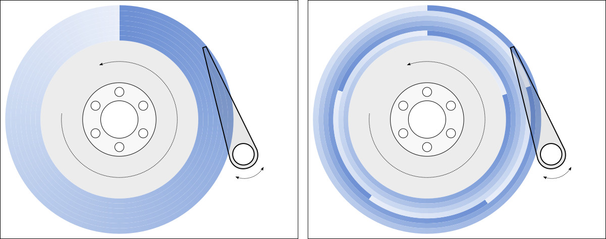
Track layouts. Traditional “head-first” layouts arrange tracks into cylinders so that sequential accesses will change heads and access all surfaces before moving the heads to the next cylinder. Newer “seek-first” layouts first move the head to the adjacent track for some distance before switching to the next surface. There are many more possible variations that are not shown.
If a hard drive only has one recording surface, there are two reasonable ways to arrange tracks onto the surface: Outside to inside, or inside to outside. When a drive has multiple recording surfaces, there are many more ways to arrange the tracks onto surfaces. Prior work has given names to some of these arrangements [3, 1], but there are more layouts in common use. I’ll attempt to extend the taxonomy to cover more of the common layouts.
After placing the first track somewhere on (the outside diameter of) the disk, there are two obvious strategies for placing subsequent tracks. Subsequent tracks could be first placed on different recording surfaces at the same radius (cylinder) before seeking to the next radius, or a group of tracks could be first placed on the same recording surface before switching surfaces. Traditionally (old drives), switching heads was faster than moving the heads, so the first option was chosen (consecutive tracks would switch heads first before changing radius). In newer drives where head switches are slower than seeking to an adjacent track, groups of consecutive tracks are placed on the same surface before moving to the next surface.
This choice leads to two classes of track layouts, which I will call “head-first” (multiple head switches before a seek) and “seek-first” (multiple seeks before a head switch) layouts.
There are two head-first layouts in common use. One layout cycles through all surfaces in the same order for each cylinder (forward, also called traditional), while the other is to reverse the order of surfaces for each cylinder (alternating, also called cylinder serpentine). By symmetry, there are two similar layouts that order cylinders from inside to outside, but I have not seen these used.
The seek-first track layouts arrange groups of tracks on the same surface before switching heads. The group size is typically much smaller than the entire surface, usually hundreds to thousands of tracks, and the group size is usually fairly regular. This group of tracks is sometimes also called a serpentine, derived from the name given to one of these layouts (“surface serpentine”).
Due to the use of serpentines (as opposed to filling an entire surface before changing surfaces), there are four common seek-first layouts. First, tracks within serpentines can always be ordered outside to inside (forward seek direction), or the order can be reversed on alterating surfaces (alternating seek direction: outside to inside on one surface, inside to outside on the next). There can also be layouts that use a reverse seek direction, but these were never observed. Second, similar to head-first layouts, the order in which surfaces are used can repeat for each group of serpentines (forward surface order), or the order can reverse after each group (alternating surface order). These two properties combine to create four options. Two of these four were given names in prior work: alternating-forward is also called surface serpentine, and forward-forward is also called hybrid serpentine.
This classification is not exhaustive. For example, the Western Digital S25 uses a seek-first layout with forward seek direction, but the serpentine size and the sequence of surfaces does not follow a regular pattern. This layout cannot be classified into any of the six layouts described above.
Prior Work
There have been many previous attempts at characterizing the properties of hard drives using microbenchmarks. This article makes another attempt because hard drives have changed over the years and there hasn’t been an attempt to make detailed measurements of so many drives spanning so many years.
Many of the prior works had practical applications in mind (as opposed to pure curiosity), and were willing to trade measurement speed for a small loss in accuracy. This article is the first I know of that attempts to make detailed measurements such as the angular position of every sector, or the size and skew of every track on a drive. Although the algorithms are not fundamentally different, prior work likely avoided exploring these because these measurements can take many hours and there is little practical benefit for applications such as performance modelling or improving data layouts in filesystems.
Many of the earlier works relied on the SCSI command set to gather information [4, 5]. This included using the SCSI Send Diagnostic command to translate logical block to physical locations, and the use of the Seek command to measure seek (not access) times. These methods do not generalize to ATA drives, and relies on drives to implement these commands, to implement them correctly, and provide information that is accurate. The existence and accuracy of these commands aren’t guaranteed because they’re not essential to the operation of a drive, which only needs to read and write. Microbenchmarks that only use reads or writes are more difficult to create, but avoid many of these limitations.
Some attempts at “black-box” microbenchmarks resulted in algorithms that worked on disks of their time, but no longer work on modern drives [2]. The Skippy algorithm in particular assumed that drives used a traditional head-first track layout.
The algorithms used here are most similar to those by Gim and Won [1]. They correctly pointed out that earlier algorithms often did not work with new seek-first track layouts, and described algorithms that did. However, their algorithms were optimized somewhat more for speed at the expense of accuracy, and not quite robust enough to handle the wide variety of odd behaviours in some drives. I saw more odd behaviour due to the wider assortment of drives tested: 17 drives from 1989 to 2015 vs. 4 drives from around 2006-2007.
What is measurable?
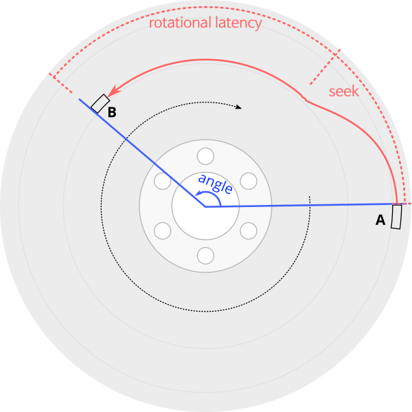
Access time measurement: Starting at A and then reading B starts with a seek, settling time after reading B’s track, then waiting for sector B to rotate under the disk head. Access time from A to B is determined by the angle between the two sectors, plus zero or more full rotations. Measuring access time gives an accurate measurement of the angle between two sectors, but not a direct measurement of the seek time.
Without internal access to the drive, measurements can only be made by sending commands and timing their response time. The basic tool I use is to measure the delay between two sector reads, with the disk cache disabled so the timings reflect the physical properties of the disk and not the cache. I did not use writes because writes destroy data on the drive, and there is less certainty on the exact time at which writes actually write to the disk media.
The time between reading two sectors depends on the distance between the sectors. After completing the first sector read (A), the time until completing the second read is the time it takes to move the disk head to the second sector’s track, waiting until the second sector arrives under the disk head, then reading the sector (B). An important observation is that this access time is the time to rotate the disk by the angle between sectors A and B, plus zero or more complete revolutions. This means that if I know the disk’s revolution time (which is easily measured), I can get a high-accuracy measurement of the angle between any two sectors (to a few microseconds or about 0.1°). This also means that it is difficult to isolate out the seek time component of the access time, because seek time affects access time only by determining how many extra revolutions are needed.
This fundamental tool of measuring the angular position of sectors can be used to build many other measurements.
- RPM: Repeatedly read the same sector (The angle is exactly 360°). This takes exactly one revolution of the disk per read.
- Angular position: By reading two sectors, the time between the two reads (modulo the revolution time) gives the angular position of the second sector relative to the first sector. This allows mapping the angular position of every sector on the disk, see where tracks start and end, and observe the amount of skew between tracks (difference in starting angular position of adjacent tracks).
- Track size: Since we can observe skew to find track boundaries (track skew occurs at track boundaries), we can find the track size for each track and the location of zones (groups of tracks with the same size). Unexpected changes in track size can also indicate tracks that have defective sectors.
- Seek time: The delay (access time) between reading one sector and another sector is the sum of the seek (including settling) time and the delay to wait until the desired sector appears under the head (rotational latency). To measure seek time, search nearby sectors to find the sector that gives a local minimum of access time. This sector is the one that appears under the head immediately after the head arrives at the target track (if the sector arrived any sooner, the head would miss the sector and would wait for one more full revolution). For this target sector, the rotational latency is near zero, making the access time roughly equal to the seek time.
- Seek profile: A plot of the seek time from a reference point (usually sector 0) to each track on the disk is a seek profile or seek curve. If we assume that a larger head motion takes longer, a seek profile can reveal the arrangement of tracks onto the surface, and also the number of recording surfaces.
- Number of surfaces: Finally! Inferring the number of surfaces essentially requires knowing the track layout.
Results Summary
The table below summarizes the measurements of the 17 hard drive models I tested. The later sections will go into more detail on each metric, how it’s measured, and general observations about each metric. Detailed results from each drive are presented on page 2.
The Toshiba DT01ACA300 and P300 are likely identical drives with different branding, so measurements across these four give some sense of how much variability there is between drives of the same model.
| Model | Capacity | RPM | Sector Size (bytes) | Sectors/Track | Tracks | Surfaces | Skew (°, rev.) | Max. seek (ms) | Avg. track pitch (nm) | Track layout |
|---|---|---|---|---|---|---|---|---|---|---|
| Seagate ST-157A 3.5″, stepper |
44.7 MB | 3602 | 512 | 26 | 3,360 | 6 | 0 | 63 | 40,000 | F or A |
| Maxtor 7405AV 3.5″ |
405 MB | 3548 | 512 | 123 – 66 | 7,998 | 3 | 93° – 100° | 30.5 | 10,000 | AF or AA |
| Seagate Medalist ST ST51270A 3.5″ |
1.28 GB | 5371 | 512 | 145 – 76 | 21,599 | 4 | 129° | 22.2 | 5200 | F |
| Seagate Medalist Pro ST39140A 3.5″ |
9.1 GB | 7209 | 512 | 297 – 169 | 72,048 | 8 | 85° | 18.3 | 3100 | F or A |
| Samsung SV0432D 3.5″ |
4.3 GB | 5399 | 512 | 403 – 231 | 24,460 | 2 | 60° (7/42 rev) | 19.4 | 2300 | F |
| Seagate ST1 ST650211CF 1″ |
5 GB | 3606.5 | 512 | 335 – 183 | 37,782 | 2 | 109.3° (17/56 rev) 116.7° (18/56 rev) |
26.3 | 280(1) | AF |
| Toshiba MK8034GSX 2.5″ | 80 GB | 5399.8 | 512 | 891 – 429 | 219,635 | 3 | 51.8° (19/132 rev) | 19.1 | 230 | AF |
| Hitachi Deskstar 7K80 3.5″ |
82 GB | 7201 | 512 | 1170 – 573 | 176,275 | 2 | 67.3° (3/16 -0.0004 rev) | 25.7 | 310 | A |
| Western Digital Caviar SE16 WD2500KS 3.5″ |
250 GB | 7204 | 512 | 1116 – 630 | 520,449 | 6 | 40° (2/18 rev) | 17.4 | 320 | AF |
| Seagate Barracuda 7200.9 ST3160811AS 3.5″ |
160 GB | 7203 | 512 | 1452 – 638 | 281,786 | 2 | 55.7° | 24.1 | 200 | FA |
| Seagate Barracuda 7200.11 ST3320613AS 3.5″ |
320 GB | 7204 | 512 | 2464 – 1200 | 329,853 | 2 | 61.3° (1/6 + 0.004 rev) | 19.9 | 170 | AA |
| Western Digital S25 WD3000BKHG 2.5″ |
300 GB | 9999.6 | 512 | 1926 – 1117 | 384,085 | 3 | 24.4° (1/15 + 0.0009 rev) | 8.1 | 100 | F* |
| Seagate Cheetah 15K.7 ST3450857SS 3.5″ |
450 GB | 15047.7 | 512 | 1800 – 1028 | 595,848 | 6 | 23.8° (1/15 – 0.0006 rev) | 7.3 | 150(2) | AA |
| Samsung SpinPoint F3 HD103SJ 3.5″ | 1 TB | 7247.1 | 512 | 2937 – 1546 | 854,135 | 4 | 72° (1/5 rev) | 17.3 | 130(3) | FF |
| Hitachi 7K1000.C 3.5″ | 1 TB | 7199.8 | 512 | 2673 – 1350 | 914,873 | 4 | 53.3° (4/27 rev) | 15.2 | 120 | AF |
| Toshiba DT01ACA300/P300 3.5″ | 3 TB | 7219.1 7200.3 7200.0 7200.0 |
4096 | 473 – 211 464 – 204 485 – 207 464 – 216 |
2,075,497 ~2,098,859 2,070,465 2,076,586 |
6 | 37.2° (3/29 rev) | 21.0 21.1 20.9 20.9 |
80 | FF |
| Toshiba X300 HDWE150 3.5″ | 5 TB | 7199.6 | 4096 | 500 – 229 | 3,279,583 | 10 | 22.5° (1/16 – 0.000008 rev) | 14.6 | 85 | AF |
1 The Seagate ST1 series manual says 105,000 TPI (tracks per inch) max, which is 242 nm per track.
2 The Seagate Cheetah 15K.7 manual says 165,000 TPI, which is 154 nm per track.
3 The HD103SJ manual says 245k TPI, which is 104 nm per track. HD103SJ was rebranded as ST1000DM005 after Seagate acquired Samsung’s hard drive business in 2011.
Rotational Speed (RPM)
The disk rotational speed is measured by repeatedly reading the same sector (sector 0). If the measurement is of a spinning hard disk, sector 0 will be read exactly once per revolution. This test is also used to verify that disk caching is disabled. If caching is enabled, the reads will hit in the cache and occur much more quickly.
Implementation Details
The cache on the Maxtor 7405AV cannot be completely disabled, so repeated reads from the same sector are serviced by the cache. Fortunately, reading a different sector is not cached on this disk, even if the sector immediately follows the first read. To compensate for this, the algorithm actually alternates between reading sector 0 and sector 1.
Sector Angular Position
The angle between any two sectors can be measured by accessing the two sectors and measuring the time between the responses of the two requests. This method usually has an accuracy of a few microseconds (around 0.1°), but depends on the drive. Any seek time (or random variation in seek time) only affects whether the second sector can be read in the same revolution, or whether extra full revolutions are needed, so we can completely remove the impact of seek time by taking the remainder after dividing the time interval by the revolution time. A map of the angular position of every sector on (a region of) the disk can be made by using a fixed sector (sector 0) as a reference point. However, since it takes tens to hundreds of measurements per sector, it is only practical to do this for small regions of the disk. Angular position plots are a powerful tool for zooming in to examine other features (such as defect management).
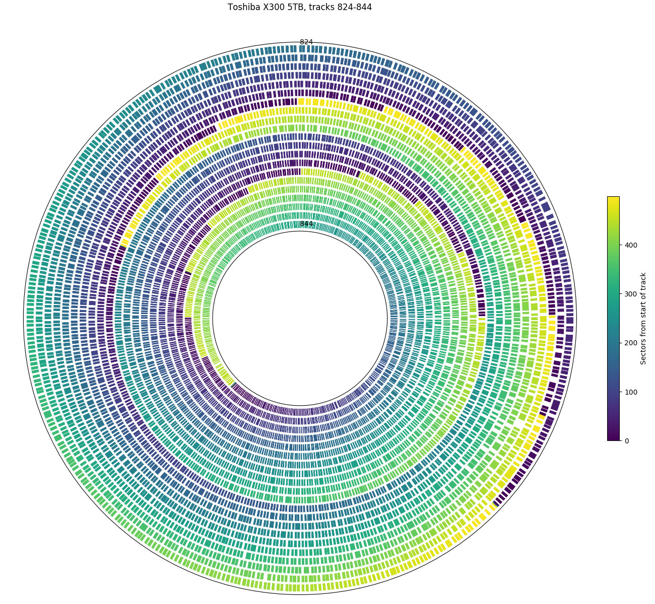
Toshiba X300 5TB: Colour scheme chosen to highlight the beginning (dark blue) and end (yellow) of each track. This shows a 22.5° track skew. Also shows a zone change, from 500 sectors per track to 460 sectors per track, with an unusual track skew at the zone boundary.

Seagate ST1 5GB: Fairly large skew of 109.3°. There appears to be a one-sector gap at the end of each track.
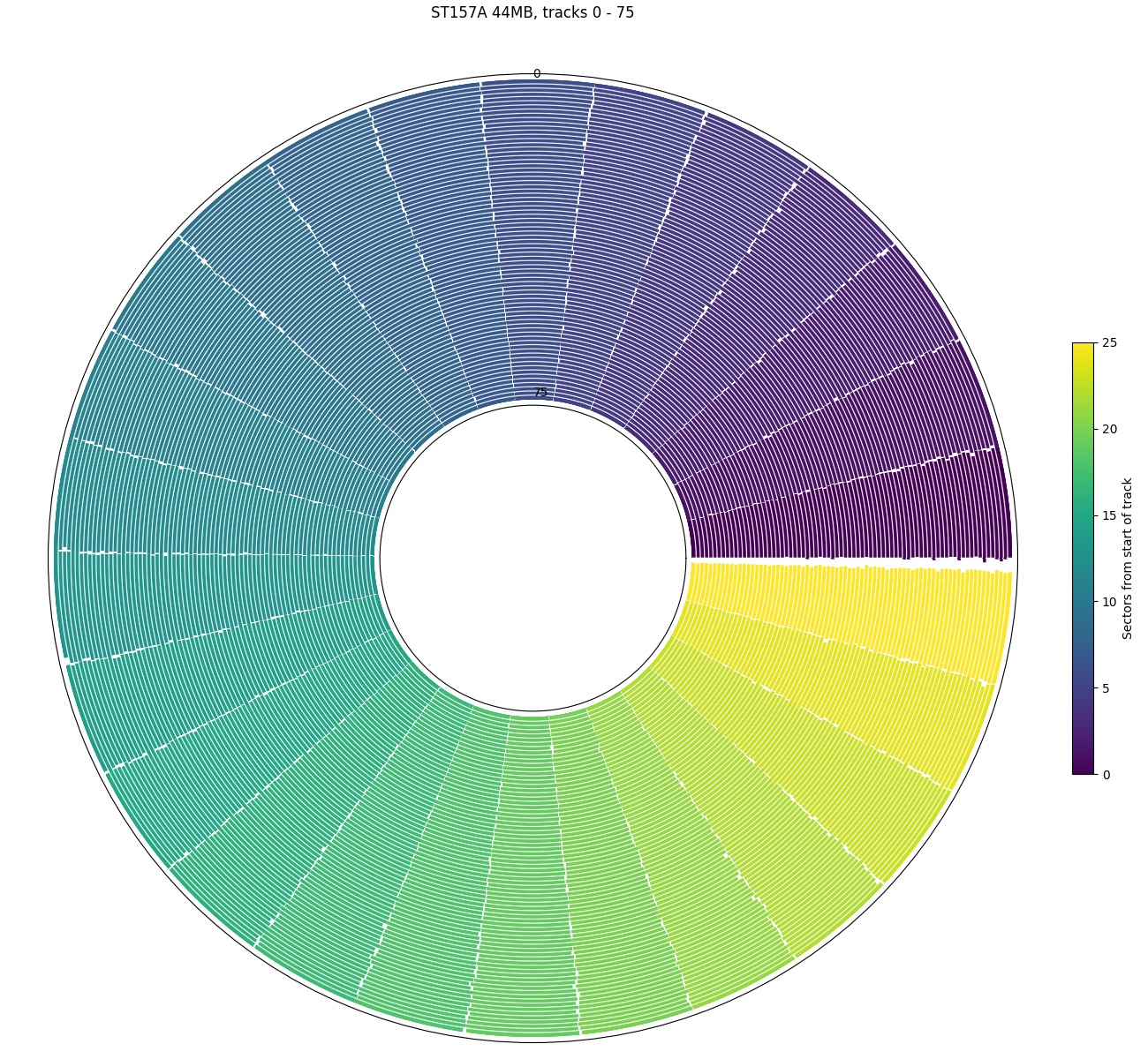
Seagate ST-157A: Only 26 sectors per track and no skew. The gap between sector 25 and sector 0 seems slightly bigger than the other sectors.
The plots above are polar plots of the angular position (Time increases in the counterclockwise direction) and track number of each sector, with the colour of each point showing the sector’s position within the track (dark is the start of a track, while yellow is near the end of a track). The colour scheme was chosen to distinguish the beginning and end of each track, which makes the track skew clearly visible. The method to find the track number of each sector is discussed in the section on finding track boundaries. These plots use track boundary information and a hole in the center to make the plot look nicer, and aren’t strictly necessary. If track boundary information is unavailable, using sector number as the radial coordinate results in a similar-looking graph, but with one big spiral instead of concentric circles and a gap (the track skew) at the end of each track. The same data can be plotted on a cartesian axis, which can sometimes be easier to read than the polar plots here.
The first plot shows tracks 824 to 844 on the Toshiba X300. It uses a 22.5° track skew: the beginning of each track is about 1/16th of a revolution later (counterclockwise) than the beginning of the previous track. This allows some time (1/16th of a rotation) to move the head and settle onto the next track after finishing reading one track before beginning to read the next track. For sequential accesses, the disk would read one track of data every (1 + 1/16) revolutions. We look at track skew in more detail in a later section.
This plot also shows a head/surface change at track 834, which is visible here as an unusually large skew. This plot shows tracks 833 and 834 as adjacent in logical track numbers, but they are actually on different surfaces and likely requires a larger seek compared to moving to an adjacent track on the same surface, which motivates the larger skew at serpentine boundaries.
The second plot is from a Seagate ST1, a 1″ hard drive in a CompactFlash form factor. Compared to the desktop and server hard drives, it has a slow 3600 RPM and still uses a large 109.3° track skew. The much larger skew gives a visually different pattern in the angular position plot. One interesting observation is that the ST1 seems to have exactly one sector of empty space at the end of every track. I don’t have any guesses on what this space is for.
The third plot is from a Seagate ST-157A, a 44.7 MB hard drive from 1989 that uses a stepper motor actuator. It has zero track skew (or perhaps more accurately, 360° of skew)! Not using any track skew likely reduces the complexity of the drive controller (which was a larger concern in 1989). However, the adjacent-track seek time is fairly large (8 ms specification, measured to be 10.8 ms including < 2.5 ms controller overhead), so the track skew would likely need to be more than 75% of a revolution (270°) anyway, and the potential performance improvement for using a non-zero skew is fairly small (10-15% sequential throughput). Also interesting is that the gap between sectors 25 and 0 appears slightly larger than between other adjacent sectors.
Implementation Details
--angpos reference,start,step,end,error (e.g., --angpos 0,0,1,10000,10)
Reference, start, step, and end are sector numbers. Error is the maximum standard error of the mean (standard deviation divided by the square-root of the number of samples), in microseconds. Use the specified reference sector, report the angular position of every step sectors from start (inclusive) to end (exclusive), and sample enough so the standard error of the mean is less than error.
The algorithm takes the average of multiple samples to improve the accuracy of the measurement. It takes samples until the standard error is below a user-specified parameter. Accuracy and runtime can be traded by changing the desired precision. There is also a speed optimization. The basic algorithm would take at most one measurement every revolution, depending on how far away the two sectors are, by visiting the source and target sectors and returning back to the source sector in one revolution. This algorithm attempts to spend two revolutions per iteration, visiting the source sector, then attempting to take as many samples as possible (of the target and later sectors), and then returning back to the source sector two revolutions later, to begin the next iteration. This algorithm can often take 10-15 samples over two revolutions, giving 5-7× speed improvement over the basic algorithm. Allowing more revolutions per iteration would further increase efficiency (with diminishing returns), but the accuracy can drop because any error in the revolution time estimate is multiplied by the number of revolutions.
Access Time
Access time is the time to move the head and read a sector, including both seek time and rotational latency. This algorithm measures the access time between a pair of sectors. It is very similar to the algorithm to measure angular position, except that the measured time is not divided by the revolution time. I normally fix the sector 0 as a reference sector, then measure the access time from the reference sector to other sectors located around the disk. This algorithm isn’t particularly novel, but it generates interesting plots when this data is plotted in polar coordinates. These plots are very similar to the angular position plots (the data point locations are actually the same), but with a different colour scheme. These plots give a visualization of what fraction of the disk area is reachable within some amount of time.
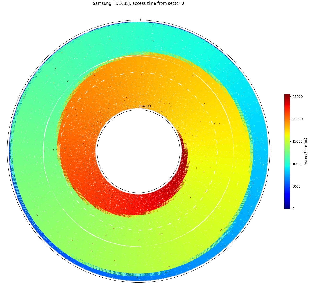
Samsung HD103SJ: Furthest sector is just over 3 revolutions away.
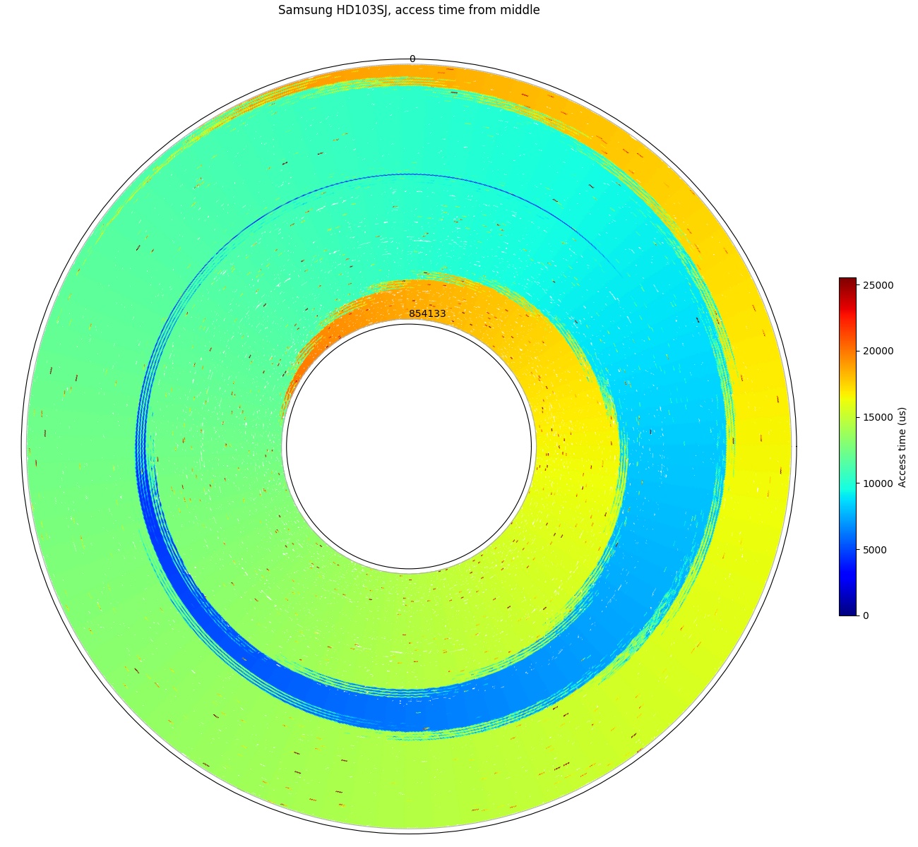
Samsung HD103SJ, access time from the middle of the disk. Furthest sector is about 2.5 revolutions away.
Above are two access time plots from the same Samsung SpinPoint F3 1TB hard drive, showing the access time from a reference sector to other points over the entire drive (tracks 0 to 854133). This plot measured one data point every few thousand sectors of the 1.95-billion sector disk. In the first plot, the reference (start) sector is sector 0 at the beginning of the drive, which is located at angle = 0 (far right) of the plot. The second plot uses sector 976762583 (middle of the drive by sector count), and the reference sector is also plotted at angle 0.
The colour swirl visually shows that the access time is mainly determined by the angular position of the target sector, while seek times determine the number of extra revolutions required to reach the target sector. Starting from the reference sector 0 (right (angle = 0), outside-most track (track 0)), the plot shows that the disk head can reach only a tiny group of outside tracks within half a rotation, about 19% of tracks after one full revolution, and reach the innermost track at just over two revolutions. In the worst case, some sectors on the innermost track need to wait one more revolution of rotational latency after the head arrives before being accessed, so the worst-case access time is ~3.09 revolutions.
In the second plot where the seek starts from the middle of the disk (by sector number, not by diameter), we see a similar pattern. Starting from the middle of the disk, the furthest seek is roughly half the distance compared to the first plot, so the worst-case access time is lower. The access time to the innermost track is slightly longer (~2.47 revolutions) than to the outermost track (~2.42 revolutions) because the middle of the disk by sector count is closer to the outside by physical distance (track number). The outer tracks store more data due to zone bit recording.
Implementation Details
--access reference,start,step,end,error (e.g., --access 0,0,1,-1,30)
Reference, start, step, and end are sector numbers. Error is the maximum standard error in microseconds. Using the specified reference sector, report the access time to every step sectors from start (inclusive) to end (exclusive), and sample enough so the standard error of the mean is less than error.
The current implementation sends the second read request only after the first one is complete, so the measurement includes OS and disk controller latency. If the intent is to measure only the mechanical performance of the drive, to get a more accurate measurement of short-distance fast accesses, it may be worth trying to send both requests at the same time so both reads can be performed without first sending the read data back to the benchmark program. This would increase the benchmark complexity (requires using asynchronous I/O and tracking the response time of each request independently), and may need to account for reordering done by the OS scheduler or disk controller (SATA NCQ or SCSI TCQ).
Because the absolute time (not modulo the revolution time) is measured, the algorithm cannot take multiple samples per revolution as done for the angular position measurement, and is limited to at most one sample per revolution. As a result, measuring access time takes several times longer than measuring angular position.
Short stroking
Looking at the two access-time plots above illustrates why short stroking the disk only gives a modest reduction in access time. Short-stroking is the practice of using only a small portion of a hard drive to keep data confined to a small (usually outer) portion of the drive to reduce the worst-case seek distance and avoid using the inner tracks that have lower transfer rates (inner tracks have fewer sectors per revolution). A significant portion of the seek time is spent in the beginning and end portions of the seek even for short seeks, as the head needs time to accelerate, decelerate, and settle. Halving the seek distance only reduced the worst-case access time by 22% (from 3.09 to 2.42 revolutions, or 25.6ms to 20.0ms). Short-stroking does not actually change seek times, but removes some longer-distance seeks from being included in the average.
For completeness, I measured the average access time for random accesses when those accesses are limited to some fraction of the disk. The graph below plots the number of reads per second (IOPS), which is the reciprocal of the access time when there are no parallel accesses (no queueing). IOPS increases when a smaller fraction of the disk is used.
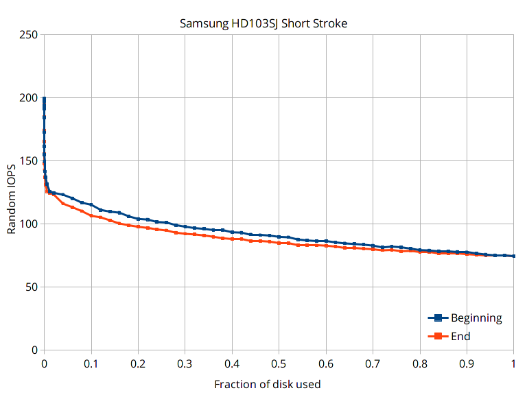
Short stroking a hard drive gives modest performance improvements by sacrificing a large amount of storage space.
The plot shows two scenarios: One where the usable region is at the beginning of the disk (the usual case when short stroking because the beginning of the disk is faster), and the other where the usable region is at the end of the disk (the slowest region). Because seek time is highly non-linear with distance (short seeks still have a high cost), the improvement in random IOPS is small unless only a very tiny fraction of the disk is used. For example, when the beginning of the disk is used, IOPS improves by about 20% when half the disk is used, 55% when 10% of the disk is used, and doubles when only 0.07% of the disk is used.
Now that flash-based solid-state drives are common, short stroking a hard drive for performance makes little sense. As of July 2019, a low-end SSD is about 3 to 4 times more expensive per capacity than hard drives, but offers 500 times higher random IOPS and double the sequential throughput.
Implementation Details
--random-access start,end,iterations (e.g., --random-access 0,-1,5000)
Start and end are sector numbers. This measures the average access time for doing iterations random accesses within the region between start (inclusive) and end (exclusive).
The algorithm reads random sectors. It measures access time, not seek time. Access time includes seek time, rotational latency (on average half the rotation period), and controller/software overhead (typically a few hundred microseconds).
Seek Time
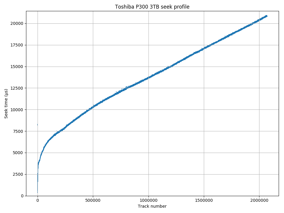
Toshiba P300 seek time vs. track number.

Access time polar plot (Toshiba DT01ACA300)
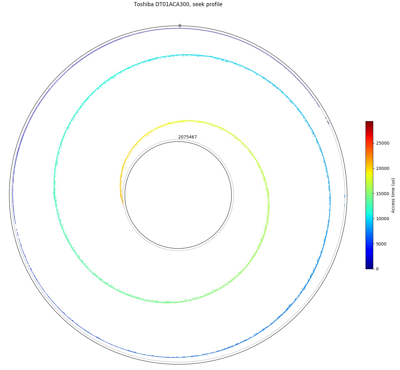
Seek profile plotted on a polar axis. A seek profile is equivalent to finding the boundary between colour regions in the acess time plot.
The seek time is the time it takes for the disk head to move to the destination track, but not including the rotational latency to wait for the target sector to rotate under the disk head. I included head settling time in the seek time because settling is really just the final low-speed fine-tuning portion of the seek, and there is no way to measure settling time separately from the seek. Seek time provides information about the radial location of a given track on the disk. Seeks of a longer physical distance usually take longer than seeks of a shorter physical distance, so seek time can be used to determine which tracks are physically closer to a reference location. I usually use sector 0 on the outer edge as the reference sector.
While it is straightforward to measure access time, seek time requires finding the sector on the target track that has the lowest access time (with near-zero rotational latency). Nisha et al. [2] describe an algorithm that measures the access times between one sector and a number of sectors near the seek target, then chooses the minimum. My algorithm improves on speed by using a logarithmic search for the sector with the minimum access time starting with big steps that decrease exponentially (the runtime is logarithmic in the number of sectors per track rather than linear). This becomes particularly important when disks have many sectors per track. I tested disks with up to 2937 sectors per track, while Nisha et al. only tested up to 356.
The seek time profile is usually plotted with seek time on the vertical axis and seek distance (number of tracks) on the horizontal axis. The diagram to the right shows an example from a Toshiba P300 3 TB drive. The seek time increases roughly linearly with distance for long seeks (when the seek time is dominated by the head moving at a high constant speed) and is non-linear for short seeks (dominated by acceleration, deceleration, and settling time).
Another way to think of the seek time curve is that it is the boundary that separates colour regions in the access time plot. The seek time is the access time of the set of sectors that have near-zero rotational latency, which are those sectors that sit on the boundary between “arriving immediately after the head arrives” and “arriving slightly after the head arrives and needing an extra revolution”. To demonstrate this, the two polar plots to the right plots the seek profile and access time data points for the same drive on the same polar axis for comparison. The seek profile is usually more useful when plotted in cartesian coordinates.
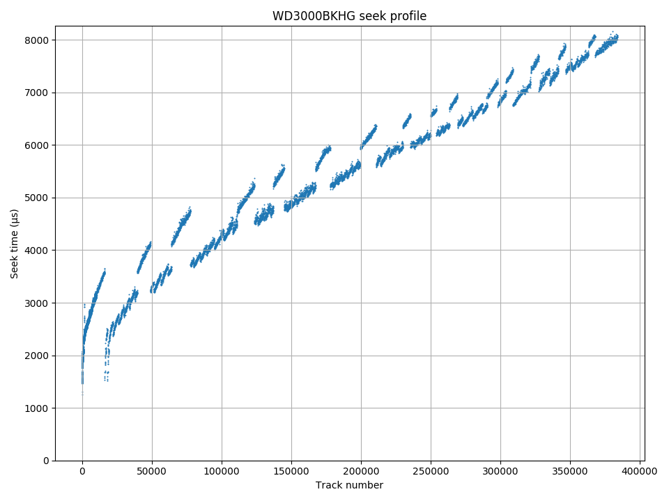
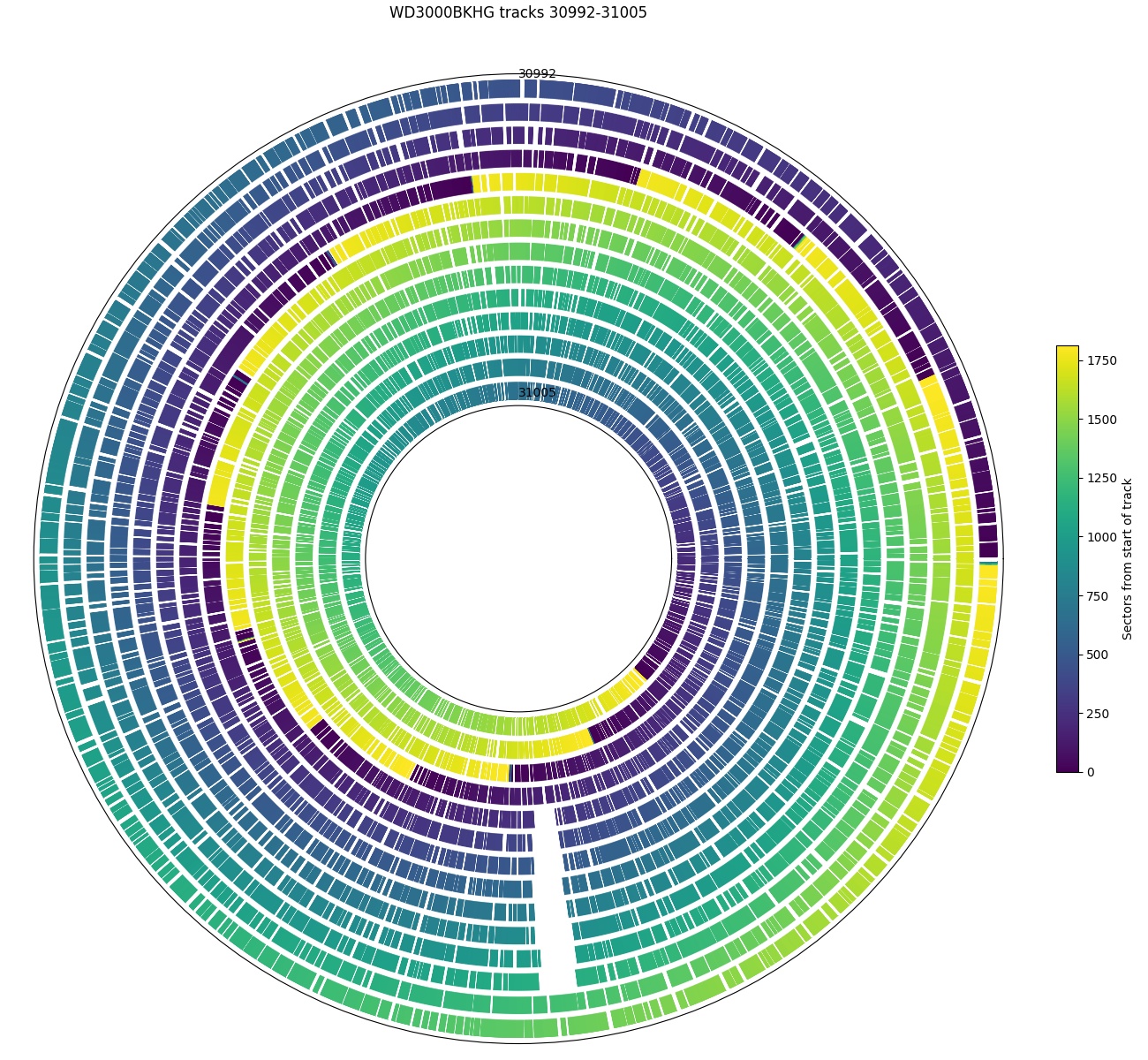
Western Digital S25: The seek profile is unusual, indicating a strange mapping between track numbers and physical location. This mapping seems quite irregular.

Samsung F3. Even when completely zoomed out, four recording surfaces are visible.
The two plots on the right are examples of slightly more complicated seek time profiles. The seek time plots for the Samsung F3 (HD103SJ) and WD S25 (WD3000BKHG) are not smooth even when zoomed out. These patterns indicate that tracks are not strictly placed from outside diameter to inside diameter, but that there are some later logical tracks that are physically closer to the outside (lower seek time) than some earlier tracks (higher seek time). These patterns give information on the track layout, which we will look at in the track layout section.
Implementation Details
The access time of a sector depends on its angular position. The algorithm to find seek time searches nearby earlier sectors to find a local minimum sector with near-zero rotational latency.
--seek-track reference,start,step,end (e.g., --seek-track 0,0,1,-1)
Reference, start, step, and end are sector numbers.
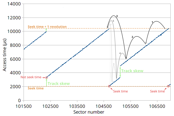
The seek time is the access time for the sector on the target track that has the lowest access time (near-zero rotational latency). This algorithm starts by measuring the access time (including the rotational latency) to an arbitrary target sector. It then measures the access time for an earlier sector, chosen to be likely on the same track but with less rotational latency. This process is repeated until the access time suddenly increases, which occurs when the target sector arrives too soon under the head and we need to wait one more full revolution. The step size is then halved and the search repeated until the sector with minimum access time is found. There is one common case where this search fails: if the optimal sector actually falls within a track skew (This is labeled as “Not seek time” at sector 102345 in the diagram). When this happens, the search will then conclude that the current track’s first sector has the lowest access time, but it actually has non-zero rotational latency because there is a physical gap between the current track’s first sector and the previous track’s last sector (the track skew). This implementation tries to mitigate this by attempting to search two adjacent tracks before reporting the seek time.
Like the access time measurement, the seek time measurement sends read requests serially and thus includes the OS and disk controller overhead.
Both the SCSI and ATA command sets contain a Seek command that might give a more direct measurement of seek time. I have not attempted to use this. This command is “obsolete” for SCSI, and I don’t know its status for ATA, nor do I know how reliably these commands are implemented in various hard drives. (Example: The Cheetah 15K.7 manual claims that both the Seek and Seek Extended commands are implemented.)
Acoustic Management
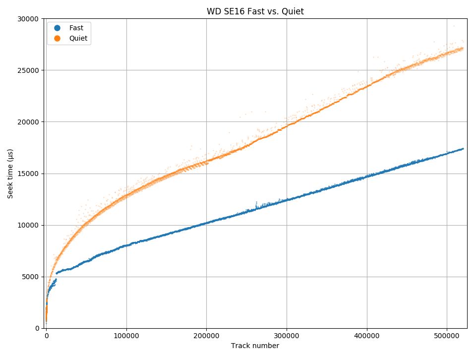
WD S25: Full-stroke seek increases from 17.4 ms to 27.1 ms in quiet mode.

WD S25: Seek time for short-distance seeks (< 2.2 ms) is not affected.
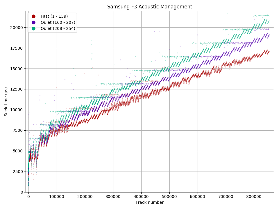
Samsung F3: Full-stroke seek increases from 17.3 ms to 21.0 ms in quiet mode
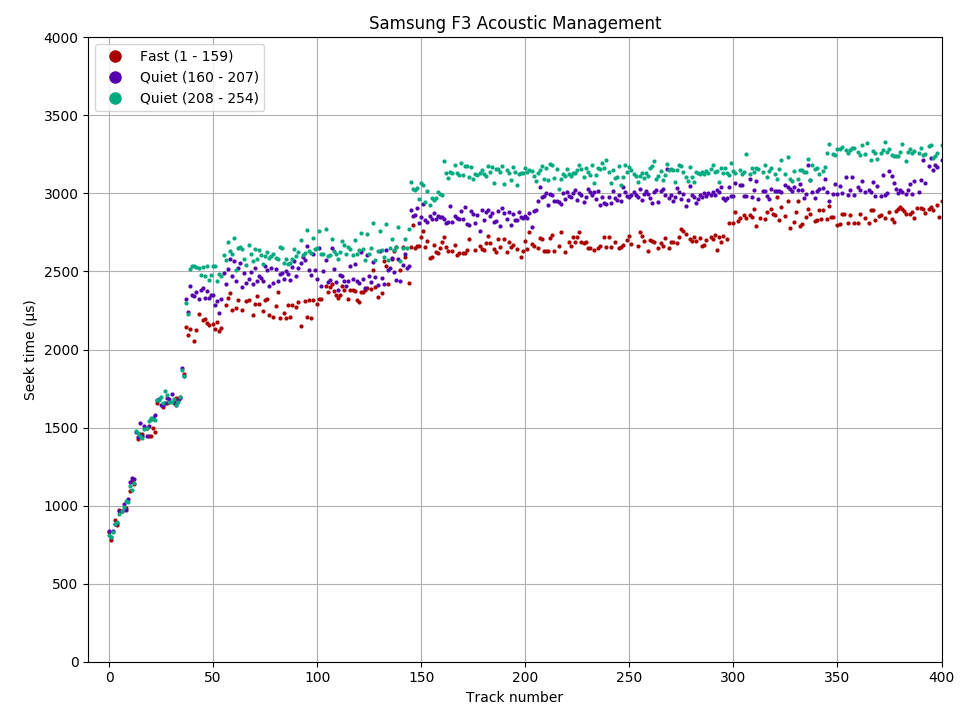
Samsung F3: Seek time for short-distance (< 2 ms) seeks is not affected.
Automatic Acoustic Management (AAM) is a method to allow the user to reduce audible noise from the hard drive in exchange for lower performance. Since most of the noise comes from moving the disk head during seeks, AAM essentially slows down seeks (increasing seek time) to reduce noise. This feature appeared in ATA-6 (2002) [6], but doesn’t seem to be implemented in many (newer?) drives.
Using the ability to measure seek time, we can see how AAM quiet mode affects seeks. The diagrams show a seek profile in both fast (default, in blue) and quiet (in orange) modes. For the WD SE16, quiet mode increased the maximum seek time by 55% from 17.4 ms to 27.1 ms. For the Samsung F3, the increase is 21% (17.3 ms to 21.0 ms). If we zoom in to the beginning of the disk, we see that the seek time of short seeks (below 2.2 ms for WD S25, 2.0 ms for Samsung F3) are unaffected. This makes sense: Short seeks are quiet even at full power, and adjacent-track seeks cannot be allowed to get slower because if an adjacent-track seek takes longer than the track skew, sequential throughput becomes halved.
Track Boundaries
Finding track boundaries means finding the sector number of the first sector of every track. Designing an algorithm to find them reliably is surprisingly difficult. A track is a group of consecutive sectors that spans around one revolution of the disk, separated by track skew. The algorithm identifies track boundaries by looking for the track skew (an unusually large change in angular position between two adjacent/nearby sectors). I’ll leave discussion of the many ways this algorithm can fail in the Implementation Details section below.

Toshiba MK8034GSX: track sizes
Toshiba MK8034GSX disk throughput benchmark. Throughput is proportional to track size (if track skew is constant).
The number of sectors per track is proportional to the sequential throughput of the disk. The drive spins at a constant angular speed, so sequential throughput varies with how much data is read per revolution. During sequential accesses, the drive reads one track of sectors every (1+skew) revolutions, so the sequential throughput can be calculated exactly from track size, RPM, and track skew. Previous work has even used this relation in reverse to compute approximate track sizes by measuring sequential throughput [1, 2]. The two figures above show a comparison between track sizes and a throughput benchmark for the same disk (Toshiba MK8034GSX), showing that they look very similar.
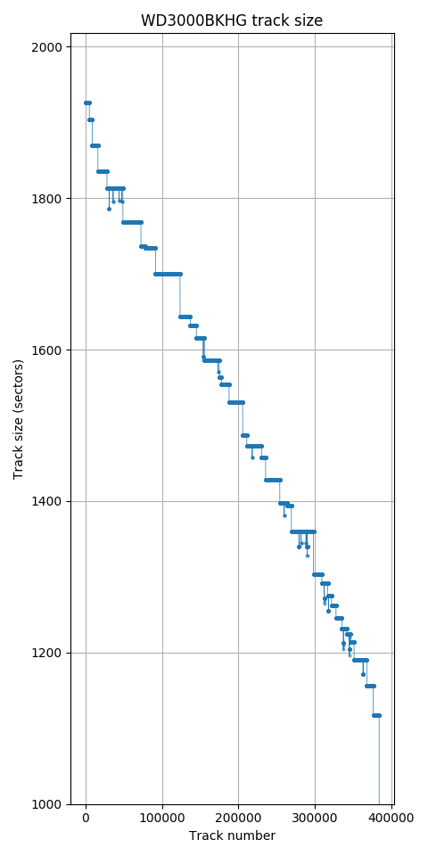
Western Digital S25 300GB. Track size monotonically decreases (except for defects).

Samsung HD103SJ 1TB. This drive switches heads/surfaces infrequently.
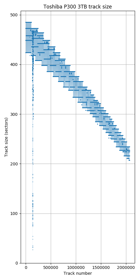
Toshiba P300 3TB. The region near track 140,000 is a region with many defective sectors causing the track size to drop.
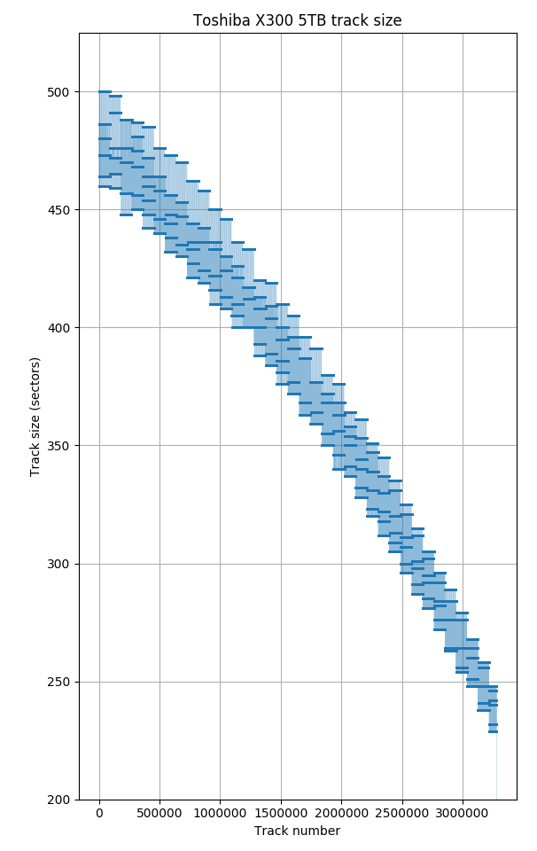
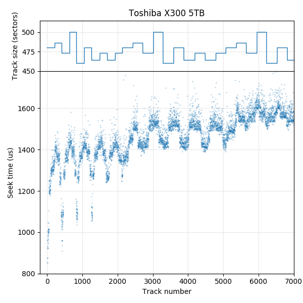
Toshiba X300 5TB.
All newer hard drives use zone bit recording, so earlier tracks have more sectors than later tracks. This sequence is usually not strictly monotonically decreasing because the number of sectors per track is often different on each recording surface, causing the track size to vary according to how tracks are arranged onto the surfaces. For the Toshiba P300 and X300, the plot looks shaded because the track size switches very frequently between several values according to which surface a track is placed on. The Samsung HD103SJ switches between surfaces much less frequently.
Although track size decreases monotonically for both the MK8034GSX and WD S25, they are actually quite different. The MK8034GSX uses a surface serpentine layout (seek first type AF, with a head change every ~115 tracks), but the track size is the same on every surface, so the track size curve monotonically decreases. The WD S25, however, uses different track sizes on each surface, but tracks are ordered by decreasing size, not by physical location. The result is a monotonically-decreasing track size curve, but highly irregular serpentine sizes causing an irregular seek profile. We will discuss this further in the section on measuring track layouts.
In the above plots, the x-axis is in units of track number (not sector number). If the track density were constant, then track number would be linearly related to the physical radius of the track. Also, if the linear bit density were constant across the disk, then the track size would be proportional to the length (and also radius) of the track. If the above two assumptions were true, I would expect to see the track size vs. track number plots to be a straight line. But almost all of the drives show a slight convex shape. Why? My guess is that this is related to the angle of the disk head relative to the track (confusingly called “skew angle”). In the (usually) middle tracks of the disk, the disk head is designed to be aligned with the track, but at the inner (ID) and outer (OD) diameter positions, the head is rotated relative to the track (because the head is mounted on a rotating arm), which causes the achievable bit density to be lower at the ID and OD. Cordle et al. [7] report a decrease of 8-10% in areal density capability (ADC) at both ID and OD compared to the middle for a PMR (perpendicular magnetic recording) disk, which seems reasonably close to the shape of the track size curve seen here. (PMR has been used in most hard disk drives since around 2006 until today, with HAMR (heat assisted) coming “soon”.)
Implementation Details
--track-bounds 0,-1
--track-bounds-fast 0,-1
In the simplest case, a track consists of a group of consecutive sectors, separated by a track skew. Thus, we can detect track boundaries by finding the location of the skew (an unusually large change in angular position between two nearby sectors). We can also assume that track sizes tend to be fairly similar (adjacent tracks differ in size by less than a few tens of percent). Unfortunately, none of these assumptions actually hold consistently across all drives and all tracks. I needed to manually fix some of the incorrectly-detected track boundaries.
Although most drives have non-zero track skew, some old drives (ST-157A) have no (or 360°) skew. While an algorithm could attempt to detect 360° of skew and treat that as a track boundary, it would be extremely difficult to distinguish this from two adjacent sectors on the same track. My current implementation does not work on the ST-157A, but fortunately it is so small that it is feasible to manually determine the track size (26 sectors per track without zone bit recording). Even for drives with non-zero track skew, there are tracks with different skew. Most drives have unusual (sometimes near-zero) skew at serpentine or zone boundaries, and skew can be fairly random when a track boundary occurs along with track slipping (defect management) or in the middle of a block of defective sectors when using sector-slipping defect management.
I implemented two algorithms. The first is a O(lg tracksize) algorithm to find a track boundary. A track boundary contains a track skew that increases the angular distance between two (logical) sectors if the two sectors cross a track boundary. The algorithm can then repeatedly split the region into two and test which half contains the track boundary (binary search) until the exact location is found. There are several speed optimizations on top of this basic algorithm. The algorithm also predicts the location of the next track boundary (track size tends to be constant within a serpentine and zone), and if the prediction is correct (which is the common case), the next track boundary can be confirmed without a binary search. Also, for large regions, it splits the region into more than two sub-regions because we can test multiple regions in the same revolution.
The second “fast” algorithm is an extension of the first algorithm, and is largely based on the “MIMD” (multiplicative increase, multiplicative decrease) algorithm proposed by Gim and Won [1], with improvements to improve robustness. Because track sizes tend to stay constant for relatively large regions, it may be profitable to not just predict the location of the next track boundary, but to predict that multiple upcoming tracks are all the same size. If the prediction is correct, we double the prediction for the next iteration, otherwise we halve the number of skipped tracks and try again. The algorithm is essentially binary-searching for zone/serpentine boundaries rather than track boundaries, so it does not need to visit every track.
In my implementation, “fast” mode is restricted to predicting exact multiples of the previous track size (Gim and Won allow an error of ±5 sectors). If the prediction is not exactly correct even for one track ahead, it falls back to the O(lg tracksize) algorithm described above to handle the change in track size. To verify the prediction, I verify that track boundaries exist at both (n-1) and (n) tracks ahead (Gim and Won only checks (n) tracks ahead). This was necessary because when track size changes, the change in track size multiplied by the number of tracks the algorithm chose to skip can be exactly a multiple of the previous track size, leading to an incorrect result. For example, if the current track size is 1000 sectors and the algorithm wants to check whether 64 tracks (or 64000 sectors) ahead is still within the same zone, it would incorrectly conclude that the zone continues for 64 1000-sector tracks if the reality were that there were 80 800-sector tracks instead. The probability of this occurring is low, but with millions of tracks per disk, I routinely saw a few incorrectly-predicted blocks for this reason. Even doing two checks per prediction does not guarantee correctness. For example, if there were two consecutive tracks that were exactly half the size of its neighbours (this is unlikely, but not impossible), both algorithms would incorrectly identify it as a single normal-sized track.
In the most extreme cases (namely, the blob of defects in one of my P300 drives), I had to resort to plotting an angular position plot of every sector in the region and identifying track boundaries manually. There were some tracks that had lost over 90% of its sectors, and the track boundary finding algorithms got hopelessly lost in those regions.
Here are two examples where the track-finding algorithm fails. The first example illustrates difficulties when there are holes of missing sectors due to defects. The animation below shows the result of running the track boundary finding algorithm ten times on a region of the disk with one large hole and some small holes scattered around. The colour scheme is chosen to highlight the first few sectors of each track in dark blue. Every run produces a different result as the algorithm often mistakes the hole for track skew.
The second example does not involve defects. On the Samsung SV0432D, the last track of each zone may not be a complete track. In this example, track 8891 is in a zone with 392 sectors per track, but the final track of the zone (8892) is only 6 sectors long. The next zone has 386 sectors per track, which is exactly 6 fewer sectors than the previous zone. An algorithm that looks for track boundaries would find one at precisely the expected location (392 sectors past the end of track 8891), not realizing that it missed a track boundary in between. This case was found by manually inspecting all of the zone boundaries because I noticed very small tracks near some of the zone boundaries.
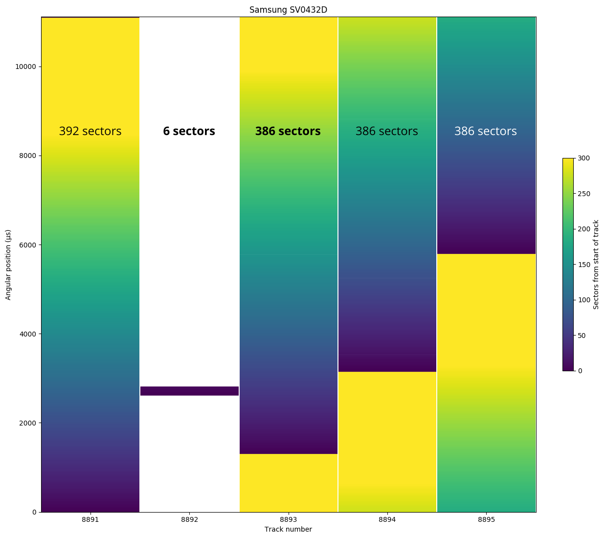
The last track of a 392-sector/track zone (6 sectors in size) plus the first track of the next zone (386 sectors) is exactly the same size as tracks in the zone (392 sectors).
Track pitch and bit density
Now that we know the track boundaries (and thus, the number of tracks), it would be interesting to try to estimate the track pitch, which is usually measured in tracks per inch (TPI). Calculating the track pitch requires knowing the physical distance between the outer and inner tracks, which cannot be measured by timing alone. This, I use photographs of the hard drives to estimate the physical size of the platters.
This table shows the approximate measurements. Using these measurements, we can calculate the average track pitch (track pitch can vary between the outer, middle, and inner tracks). For the drives I tested, track pitch ranges from 40 µm to 80 nm, or 650 TPI to 310,000 TPI.
| Model | Capacity | OD | ID | Avg. tracks per surface | Sector Size | OD track size | Avg. track pitch | OD linear density | ||
|---|---|---|---|---|---|---|---|---|---|---|
| (mm) | (mm) | (bytes) | (sectors) | (nm/track) | (TPI) | (nm/bit) | (kbpi) | |||
| Seagate ST-157A 3.5″ |
44.7 MB | 87 | 43 | 560 | 512 | 26 | 40,000 | 650 | 2600 | 10 |
| Maxtor 7405AV | 405 MB | 91 | 35 | 2666 | 512 | 123 | 10,500 | 2400 | 570 | 48 |
| Seagate ST51270A | 1.28 GB | 91 | 35 | 5400 | 512 | 145 | 5200 | 4900 | 480 | 53 |
| Seagate ST39140A | 9.1 GB | 91 | 35 | 9006 | 512 | 297 | 3100 | 8.2k | 240 | 100 |
| Samsung SV0432 | 4.3 GB | 91 | 35 | 12230 | 512 | 403 | 2300 | 11k | 170 | 150 |
| Seagate ST1 ST650211CF 1″ |
5 GB | 23 | 12.5 | 18891 | 512 | 335 | 280 | 91k(1) | 53 | 480(1) |
| Toshiba MK8034GSX 2.5″ | 80 GB | 62 | 28 | 73212 | 512 | 891 | 230 | 109k | 53 | 480 |
| Hitachi Deskstar 7K80 | 82 GB | 91 | 35 | 88138 | 512 | 1170 | 310 | 81k | 60 | 430 |
| Western Digital SE16 | 250 GB | 91 | 35 | 86742 | 512 | 1116 | 323 | 79k | 63 | 410 |
| Seagate 7200.9 | 160 GB | 91 | 35 | 140893 | 512 | 1452 | 200 | 128k | 48 | 530 |
| Seagate 7200.11 | 320 GB | 91 | 35 | 164927 | 512 | 2464 | 170 | 150k | 28 | 900 |
| Western Digital S25 WD3000BKHG 2.5″ |
300 GB | 62 | 36 | 128028 | 512 | 1926 | 100 | 250k | 25 | 1000 |
| Seagate Cheetah 15K.7 ST3450857SS 3.5″ |
450 GB | 66 | 37 | 99308 | 512 | 1800 | 150 | 174k(2) | 28 | 900(2) |
| Samsung SpinPoint F3 HD103SJ 3.5″ | 1 TB | 91 | 35 | 213534 | 512 | 2937 | 130 | 194k(3) | 24 | 1100 |
| Hitachi 7K1000.C 3.5″ | 1 TB | 91 | 35 | 228718 | 512 | 2673 | 120 | 207k | 26 | 970 |
| Toshiba P300 HDWD130 3.5″ | 3 TB | 91 | 35 | 345078 | 4096 | 485 | 80 | 313k | 18 | 1400 |
| Toshiba X300 HDWE150 3.5″ | 5 TB | 91 | 35 | 327958 | 4096 | 500 | 85 | 298k | 17 | 1450 |
1 The Seagate ST1 series manual says 105,000 TPI (tracks per inch) max. It also says linear density is 651 kbpi max.
2 The Seagate Cheetah 15K.7 manual says 165,000 TPI. It also says linear density is 1361 kbpi max.
3 The HD103SJ manual says 245k TPI.
For the three drives where the manual lists a track pitch number, two of my estimates show a significantly lower track density that the published number, by up to 20%. I do not know the reason for the difference, but possible causes include the manual publishing the maximum density of the densest region of the disk while I compute the average, or that I have over-estimated the physical area of the platter that is actually used for data (for example, if the platter were capable of more storage than what was productized).
I can also use the same data to compute an estimate of the linear bit density for a particular track. Since we know the number of sectors per track, we can calculate the bit density of the outer track using the estimate for the outer diameter. For example, if the OD of the Toshiba X300 is 91mm and it has 500 sectors/track, this leads to about 57,300 user data bits per millimeter, or 1 user data bit per 17nm. The physical bit density is probably another 15-20% greater to account for space for the servo sectors, inter-sector gap, sync, data address marker, error correction code, and line coding of the user data.
For the two cases where a linear density specification was listed, the specification is far higher (by up to 50%). I can’t explain most of this gap. Some possible explanations include the outer track not having the highest linear density, or something to do with average density vs. maximum, which is known to be significantly different [8].
Track Layout and Number of Recording Surfaces
After all this work, we finally have enough information to determine the track layout and number of recording surfaces (and platters) of the disks. The simple question of how many platters a hard drive contains turned out to be surprisingly hard to measure.
The graphs below plot both the track size and seek profile charts with a shared x-axis. The graphs show only the first few thousand tracks. The track size plot shows changes in the track size that indicate when head or zone changes occur, because a head change can also change the track size if the other recording surfaces has a different track size. Changes in track skew (not plotted here) can also be used to locate head changes, which is especially useful for drives that use the same track size on all surfaces. The seek profile gives an approximation of the radial location of the track. Tracks located nearest the outer edge have lower seek times. This is the same method used by Gim and Won to find track layouts [1].
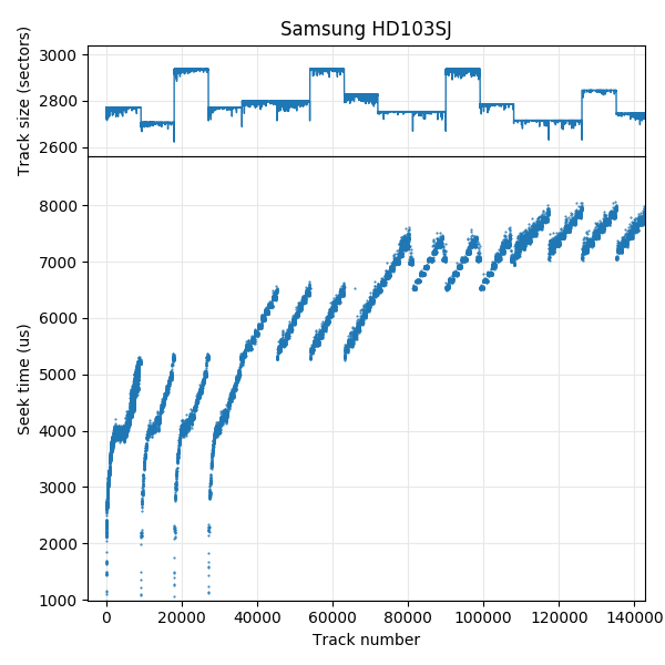
Samsung HD103SJ: 4 recording surfaces. This disk switches surfaces infrequently (note the x-axis scale), and head switch coincides with zone boundaries.
Toshiba X300: 10 recording surfaces.

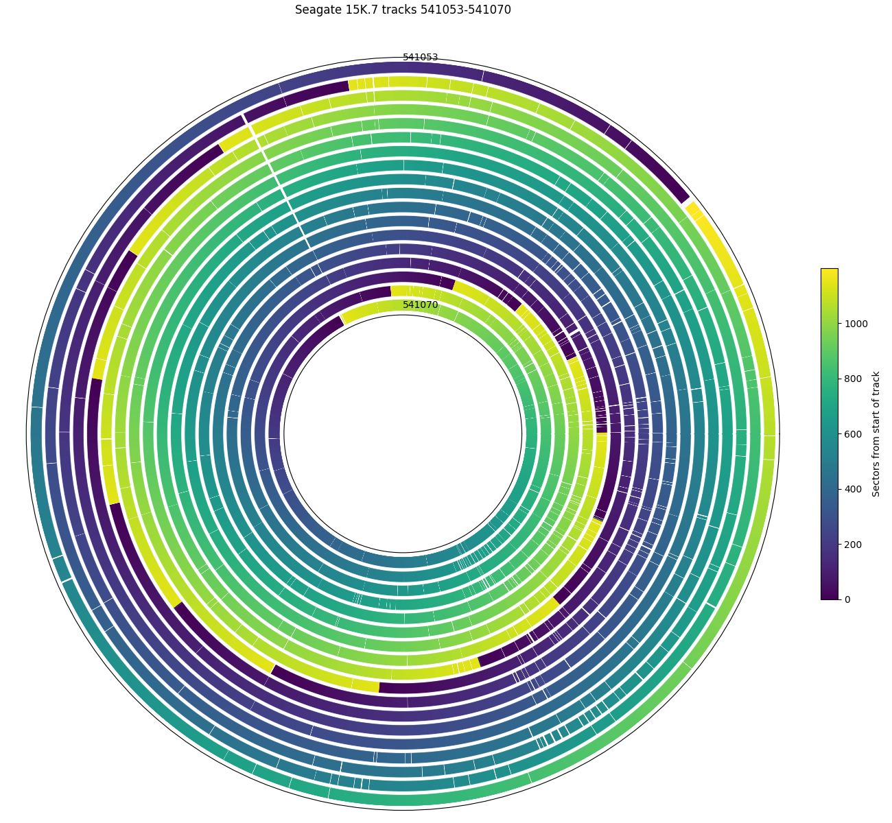
Seagate 15K.7: 6 recording surfaces.
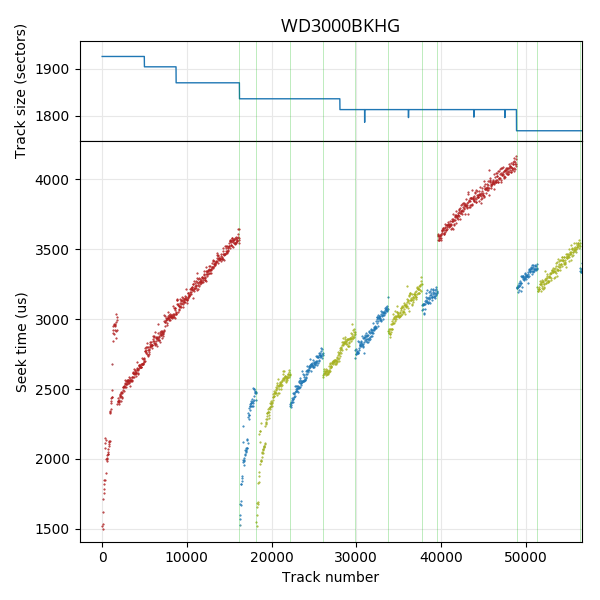
Western Digital S25: 3 recording surfaces. Each surfaces is shown in a different colour in the seek profile.
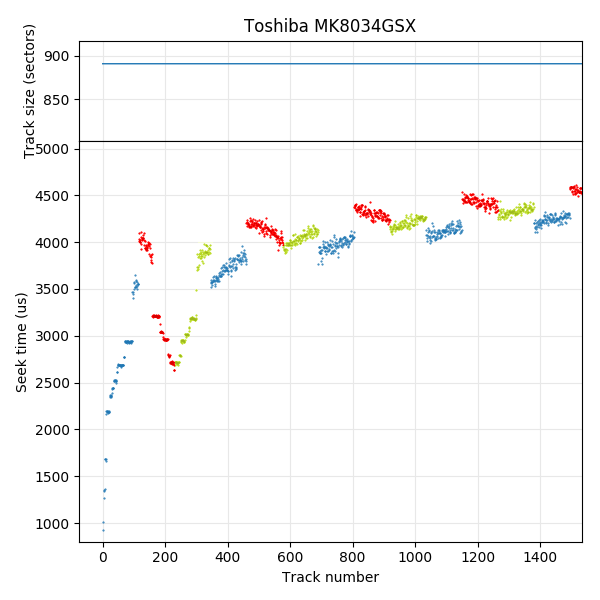
Toshiba MK8034GSX: 3 recording surfaces.
The graph for the Samsung HD103SJ is fairly easy to read. It shows four recording surfaces, each of which has a different track size. Starting at the beginning of the disk, tracks are filled on one surface from outside towards the inside (seek time increases from track 0 to track 9235), then moves to the outer track of the next surface. This pattern repeats four times (indicating four surfaces) before moving further inwards. The next group of four zones starts at track 36009. Looking at the track size (upper) subplot, we can see that the track layout cycles through the four surfaces in the same order: The third surface has the highest density. The assumption here is that the “quality” can differ between recording surfaces, but that the quality of the same surfaces changes slowly. Regions of the same size are more likely to be on the same surface and adjacent than zones that differ in track size. Also, all serpentines have tracks that are ordered from outside to inside. This drive thus uses a seek-first, forward seek order, forward surface order layout (“seek first, FF”).
The Toshiba X300 5TB drive has 10 recording surfaces, each having different track density. The track layout is different than the HD103SJ. Tracks are filled from outside toward inside on the first surface, but filled in the reverse direction on the next surface (alternating seek order). The seek profile looks like groups of five upside-down U shapes. The 10 surfaces are cycled through in the same order (the fourth surface has the highest density). This drive uses a “seek first, AF” layout.
The Seagate 15K.7 (with 6 recording surfaces) appears to use a similar track layout as the X300, showing upside-down U shapes in the seek profile. However, the track size plot shows that it cycles through the surfaces in a different order. Each group of 6 serpertines are mirrored, which indicates surfaces 1 to 6 are used for the first group of serpentines, followed by surfaces 6 to 1 in reverse order (alternating surface order). This drive uses a “seek first, AA” layout.
The Western Digital S25 has three recording surfaces. For clarity, I coloured each recording surface with a different colour in the seek time profile. The seek profile looks irregular but the track size plot monotonically decreases. It appears the strategy used here is to always have a monotonically-decreasing track size by varying the order in which physical tracks are used. The few tracks that have slightly fewer sectors than its neighbouring tracks is caused by skipping over defective sectors. The surface with the highest track size is used first, with the first 16208 tracks all placed on this surface. The other two surfaces are used starting at logical track 16208, and returns to the first surface near track 39600. This drive uses a seek-first, forward seek direction layout, but no regular pattern in the surface order.
As mentioned in the track boundaries section, the Toshiba MK8034GSX also has monotonically-decreasing track sizes. As shown here, the track layout is actually the same as the Toshiba X300, except with only 3 surfaces (seek-first, AF). The reason the track sizes decrease monotonically is because all surfaces use the same track sizes and zone boundaries. In contrast, the WD S25 uses surfaces with different track sizes, but the tracks are reordered to make logical track sizes monotonically decreasing.
Track alignment across surfaces
The seek profile shows an indirect measurement of the distance between a reference point (sector 0) and other tracks on the disk. On drives with multiple recording surfaces, the plot can be discontinuous due to a serpentine-type layout, where a non-adjacent track (hundreds of tracks away) is actually physically nearby (minimal head movement) on a different surface.
One interesting way of interpreting this information is to ask the question: How well are tracks on one surface aligned to tracks on different surfaces? In classical track layouts, it was assumed that head switches (electrical) are faster than an adjacent-track seek (mechanical), so consecutive tracks are laid out in cylinders, switching heads multiple times before moving the head to the adjacent cylinder. But with increasing track density, tracks may have become too difficult to align on different surfaces.
As an example, the seek profile for a 3 TB Toshiba P300 show that tracks can be poorly aligned between surfaces. Below is the seek profile for the first 1100 tracks the disk, which spans the first 8 serpentines (on 6 surfaces). In the seek profile plots above, I used sector 0 as the reference point. Here, I created an animation where I varied the reference point between track 0 through track 140 (spanning exery track in the first serpentine on the first surface). The reference location is indicated by the arrow. I also highlighted serpentine boundaries to make them easier to see. Because there are 6 surfaces, there are 6 minimum peaks, one per recording surface. The location of the peaks indicate which logical tracks are physically closest to the reference point. This allows seeing whether serpentines on different surfaces are aligned to each other, by seeing whether the peak in each serpentine is in the same relative location in every serpentine.
On this disk, the serpentines are not well-aligned. Logical track 0 of the disk is physically closest to track 38 of the second serpentine, track 26 of the third, track 63 of the fourth, track 20 of the sixth, and is 20 tracks before the start of the fifth serpentine. This suggests that if we attempted to organize these serpentines into cylinders, a head switch would likely also come with a seek of several tens of tracks due to misalignment between surfaces. With an average track pitch on this drive of about 80 nm, this misalignment is somewhere around 2 µm. This data does not show what causes the misalignment. It could be variation in the radius of the servo track initially written to the disks, or it could be the heads in the head stack assembly being not perfectly aligned, or perhaps there simply was no attempt to closely align them because a seek-first track layout is less sensitive to head switch time.
This plot also shows that a head switch alone (if minimal seek is needed) is still faster than an adjacent-track seek. The minimum peak located at the reference track involves no seek, while the two points immediately before and after it are single-track seeks. These single-track seeks take longer than the access time to the physically-nearest track on a different surface.
In conclusion, while it is still true that a head switch is faster than an adjacent-track seek, track density has increased so much that it is impossible to align tracks into cylinders, so a head switch is necessarily accompanied by a seek much greater than one track away. This explains why all newer drives use some kind of seek-first layout.
Track Skew
Track skew is traditionally defined as the angle between the starting sector of one track compared to the starting sector of the previous track. I chose to measure the starting sector of each track relative to sector 0. Knowing the absolute start position of each track can show whether the skew is exactly a fraction of a revolution or differs slightly. This is interesting because I think it gives some information about how the servo information was initially written to the blank surface, though I don’t know enough about servo writing to understand its significance.
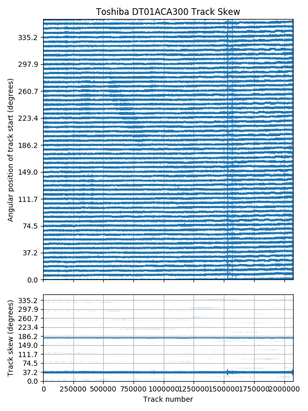
Toshiba DT01ACA300: Track skew is exactly 3/29 revolutions.
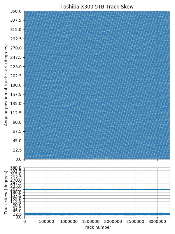
Toshiba X300: Track skew is not exactly 1/16 revolution.
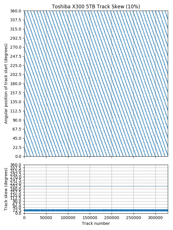
Toshiba X300, zoomed in to first 10% of the disk. Track skew is slightly less than 1/16 revolution, drifting by about 28 revolutions over 3.28 million tracks (or about -0.003° per track).
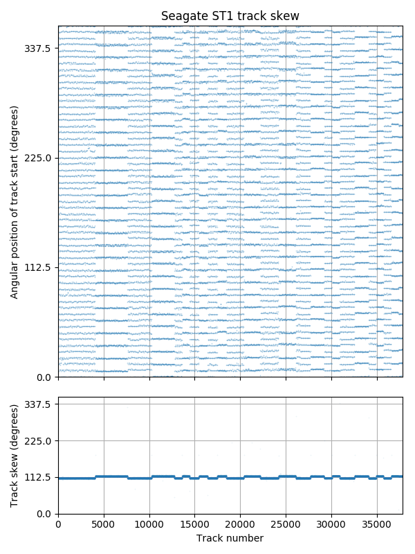
Seagate ST1: Different skew on each side of the disk (17/56 and 18/56 revolutions)
Each of the plots above have two sub-plots. The top sub-plot shows the angular position of the beginning of each track on the disk, while the bottom shows the track skew of each track (the difference in start position between adjacent tracks). The two sub-plots are two views of the same data.
The first plot above (Toshiba 3TB DT01ACA300) shows a drive that uses a skew of exactly 3/29 revolutions (~37.2°). The plot forms a set of near-horizontal lines, drifting by about 2° over the entire disk. But why are there 58 horizontal lines instead of 29? Adjacent surfaces have track start positions that are shifted by an odd multiple of 1/58 revolutions (29/58 = 180°). The bottom sub-plot shows that most of the track skews are 37.2°, but that 180° is also common. The 180° skews occur at serpentine boundaries when the next track moves to a different recording surface. There are also a small number of skews of different values. I think many of these are due to track or sector slipping, where the track start positions still follow the sequence of the real physical tracks, but some tracks are unused and skipped over.
The next plot (Toshiba X300 5TB) shows no horizontal bands in the track skew plot because its skew is not exactly a small fraction of a revolution. The bottom sub-plot shows that 22.5° (1/16 rev) and 202.5° (9/16 rev) are common skews. The third plot zooms in further, showing the first 10% of the disk. Now it is clear that the skew is slightly less than 1/16 revolutions. We can also see that the track start positions drifts by about 45/16 revolutions in this plot, or 28 revolutions over the disk. I don’t have a plausible explanation for what causes this slight drift, nor what advantages/disadvantages it might have. I suspect it depends on the method used to write the servo information [9], but I know very little about servo writing.
The fourth plot shows the Seagate ST1 5 GB microdrive. It is a 1-platter, 2-head drive, and uses a different skew on each side! One side uses 17/56 revolutions (109.3°) while the other uses 18/56 (115.7°).
Implementation Details
--access-list 0,30 < track_boundaries.txt
To measure track skew, we need to know the start sector of each track. The start sector of each track uses the output of the track bounds algorithm (previous section).
Although track skew is often defined as the start of a track relative to the end of the previous track, this algorithm measures the absolute angular position (i.e., relative to sector 0) of the starting sector of every track.
Defective Sectors
With hard drives having millions to billions of sectors, each only tens of nanometers in size, it is inevitable that there will be defects on the disk surface at manufacture time. Different drives take different approaches to manage these defects.
In some early drives, defects were “managed” by notifying the user. For example, the ST-157A manual says “A label is fixed to the drive listing the location of any media defects by cylinder, head and bytes from index”. The stickers that would be needed for a modern drive with hundreds of thousands of defects would be too expensive. With larger disks and more defects, the disk controller needs to silently skip over defective sectors (at a tiny impact to performance). Two common methods to skip over defects are sector slipping and track slipping. Sector slipping allows mapping consecutive logical sector numbers to non-consecutive physical sectors when skipping over defective physical sectors. When reading sequential logical sectors, defective sectors causes a small delay of a few sectors, but does not require extra seeks. Track slipping is similar, except that whole tracks are skipped.
How can the defect management method used by each hard drive be detected? Sector slipping causes the track length to be reduced by the size of the number of defective sectors skipped over. These can be fairly easily noticed when looking at the track size plot. In a defect-free drive, all tracks in a zone are the same size (straight horizontal line), but tracks with holes tend to show up as a group of smaller tracks within a zone. The region of interest can then be more closely examined by plotting the physical angular position of every logical sector in the region. Defective sectors that are skipped over appear as holes, and are especially visible if the hole spans multiple tracks at the same angular position. Because media defects are a physical (not logical) phenomenon, they cause holes in groups of sectors located physically near each other, ignoring logical effects such as track skew.
Sector slipping
The figures below show example sector-slipping holes for several drives. I have observed sector slipping holes in a majority of the drives. On most disks, holes are infrequent (10s to 100s per disk?) and small (a few sectors), but the Toshiba 3TB (P300 and DT01ACA300) drives seem to have more holes and much bigger holes with some holes spanning more than 90% of a track. These manufacturing defects don’t seem to have affected reliability, as none of my four drives have developed any new defective sectors during use (between 13,000 and 30,000 power-on hours so far). The only real effect is in reduced performance in the regions with holes, and that amounts to no more than hundreds of thousands of sectors out of 733 million.

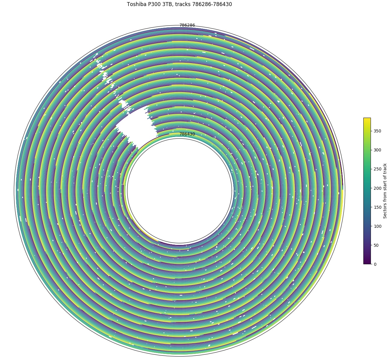
Toshiba P300: There is a big hole and a scattering of smaller holes spanning many tracks. The hole may look big, but 35 tracks is only about 2.8 µm.
A second Toshiba P300: There is a big hole here too, but overall there are fewer holes on this disk than the first P300.
Western Digital S25: There is a 27-sector hole spanning roughly the same angular positions over 8 tracks (~0.8 µm).
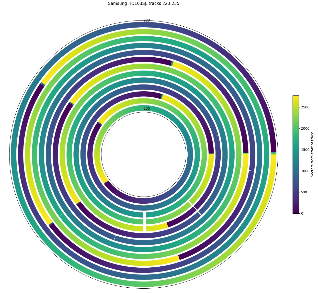
Samsung F3: There are a few holes here, the biggest of which is in tracks 231-233 (~0.4 µm).
Seagate 15K.7: There is a 2-sector hole spanning 11 tracks (~1.6 µm).
Track slipping
Track slipping is harder to find and even more difficult to verify. If a drive uses only track slipping, then all tracks in each zone contains the expected number of sectors with no exceptions. However, track slipping can cause the size of a serpentine to be smaller than expected. The easiest way to notice track skipping is the existence of an unusual track skew within a serpentine. Track skew between adjacent tracks within a serpentine tends to be constant, with larger skews occurring only at zone/serpentine boundaries (to accommodate a head switch or a larger seek). An unusual skew within a serpentine often indicates some skipped tracks. Verifying that the unusual skew is actually caused by skipped tracks is difficult. Skipped tracks cause a hole in the radial direction only (so measuring angular position doesn’t work). Radial distances can be measured using seek time (further seek → longer time), but because the seek distance to seek time relation is highly non-linear and varies for each drive model, it is difficult to accurately count the number of skipped tracks.
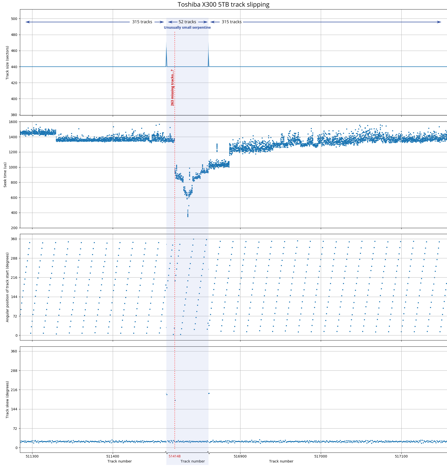
Toshiba X300 track slipping. This diagram shows three physically-adjacent serpentines on the same surface side by side (thus, the x-axis is discontinuous). There appears to be around 263 missing tracks (~22 µm) at track number 514148, causing an unusually small serpentine (52 tracks instead of 315) and an unusual track skew (177°) at the location of the skipped tracks. The seek time profile is asymmetric because of the missing tracks.
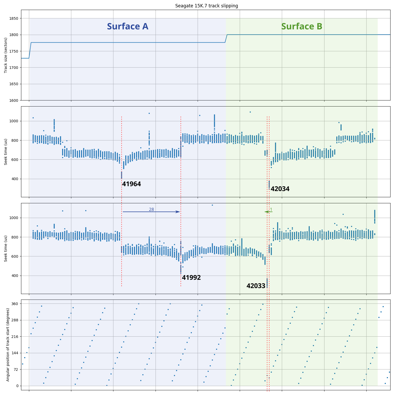
Seagate Cheetah 15K.7 track slipping. Around 28 slipped tracks (~4 µm) between tracks 42033 and 42034. Trying to measure the number of skipped tracks using an adjacent defect-free surface suggests 27 slipped tracks, but looking at the pattern of track starting positions (skew) suggests 28 missing tracks.
The figures above show two examples of track slipping and my attempt at counting the number of skipped tracks. In the first plot (Toshiba X300), there appears to be around 263 skipped tracks between logical tracks 514147 and 514148. The second plot (Seagate 15K.7) shows around 28 skipped tracks between (logical) tracks 42033 and 42034 (on “Surface B”).
The X300 plot shows three physically-adjacent serpentines on the same surface, with the middle one shaded blue. The logical track numbers are discontinuous because serpentines on the other 9 surfaces are omitted from the plot. In the top pane, track size is a constant 440 sectors, which indicates that there is no zone change. The middle serpentine size is much smaller than the usual 315-track serpentines in this region of the disk. The two spikes are left over from the unedited plot where track size changes when moving to a logically-adjacent serpentine on a different surface, which has been cut out. The second pane shows a seek profile with a reference sector somewhere inside the middle serpentine. If these three serpentines contained only physically-adjacent tracks, one would expect that the seek profile would be symmetric, but there appears to be a big section of the seek profile curve cut out between tracks 514147-514148. The third and fourth panes show track skew (angular position of the starting sector of each track, and skew relative to the previous track), showing that there is a discontinuity to the skew pattern at the same location. All three observations point to a discontinuity after track 514147, containing (315-52 = 263) physical tracks that are hidden.
The Seagate 15K.7 plot shows a different method for detecting missing physical tracks. We’ve already seen above that the seek profile plot can be used to compare radial positions between recording surfaces, which was used to observe the alignment of tracks between different surfaces. Here, I use the same method for a different purpose: I can measure physical radial distances on one surface by counting tracks on a different surface, by assuming track densities at the same radius are the same on different surfaces. In this plot, I show two adjacent serpentines on different surfaces (labeled Surface A and B in the plot), along with some suspected skipped tracks between track number 42303 and 42304. The second and third panes of the plot show seek profiles with the reference sector set to track 42034 and track 42033, respectively. The first clue that there are missing tracks is that both seek profiles are asymmetric and appear to have been cut off at tracks 42033-42034.
We can use seek profiles to measure radial distances between different surfaces. The two seek profiles show that track 42034 on Surface B is physically closest to track 41964 on Surface A, while track 42033 is closest to track 41992. If there were no skipped tracks, we would expect that moving the head a distance of one track on Surface B would also move the head by approximately one track on Surface A. Instead, a “one track” distance on Surface B was actually a 28-track distance on Surface A, which suggests 27 missing tracks on Surface B. Surface A (assumed defect-free) is being used as a ruler to measure physical distances on Surface B. Following the discontinuity of the skew pattern (bottom pane) between tracks 42033 and 42034 actually suggests there may be 28 tracks missing. In this particular example, I trust the skew pattern more, so I think 28 missing tracks is more likely than 27, but I have no way of proving it.
Missing physical tracks are difficult to detect and verify, but I’ve used two examples to show that it is possible to identify missing physical tracks and the approximate number of tracks missing. Using four independent observations increases confidence in the result: serpentine size change compared to neighbours, asymmetric or cut-off seek profile, using another recording surface as a ruler, and looking at discontinuities in the track skew pattern.
Microbenchmarking Challenges
This section is a short discussion of some of the challenges I encountered while designing this set of microbenchmarks.
Disk cache and lookahead must be disabled
My microbenchmarks assume that read commands will actually be serviced by reading the disk, and not the cache. Some previous work [2] tried to get around this by using writes instead of reads and assuming writes must wait until data reaches the disk (for safety against power loss). There are standard commands to disable caches on both ATA and SCSI disks, and these commands were functional on all but one of the drives I tested. The Maxtor 7405AV has a cache that cannot be disabled, but it appears that the cache only caches repeated reads to the same sector, so it was easy to work around this behaviour. Thus, I could use reads and avoid many of the other problems with writes (avoiding higher settling times for writes, losing the data on the disk, and never being completely certain of the exact time when data reaches the disk media).
SAS controllers come in two types: HBA and RAID. Only HBA will work.
A SAS RAID controller allows the OS to see the RAID array, but does not allow sending SCSI commands directly to the disk drives. That means it is impossible to turn off the disk cache. A simpler HBA (Host Bus Adapter) is required. A HBA simply attaches the disk to the system, much like I’m used to with IDE and SATA drives.
All microbenchmarks make assumptions about the thing being measured. These assumptions don’t always hold.
These assumptions are especially likely to be wrong if the thing you’re measuring is newer than your algorithm. The algorithms from previous work [1, 2] generally did not work unmodified on all of the wide variety of drives I tested. Indeed, even my algorithms do not work flawlessly on all of the drives, despite a lot of tuning effort, and I expect my algorithms to work even less well for drives I haven’t seen before.
The “Skippy” algorithm proposed by Nisha et al. (from 1999) [2] assumed that tracks are laid out in cylinders using one of the head-first track layouts. As we’ve seen, nearly all disks after around 2000 no longer used this style of track layout. The newer algorithms from Gim and Won (2010) [1] generally still work, but some of their optimizations do not work reliably. Their zone-finding algorithm assumes that tracks within a zone or serpentine are all the same size and change infrequently, but in modern disks with sector slipping, track sizes can change very frequently, which can produce an occasional incorrect result. Their zone-finding algorithm skips over large groups of tracks at a time, assuming the track size doesn’t change and then verifies whether the target is still a track boundary, and concluding that the entire group of tracks still have the same size. This fails when the total number of missing sectors (e.g., due to sector slipping) in a group of tracks is exactly a multiple of the assumed track size. This becomes more common with bigger drives (I tested up to 5 TB, they tested up to 320 GB) and drives with more track size variation.
My algorithms also make assumptions, and these can also fail:
- I assume a hard drive contains a stack of spinning disks, data is stored in concentric tracks (not spirals) and sectors, and that there is one head stack assembly where one head can be used at a time. I have yet to see a hard drive that is a counter-example, but there have been the occasional suggestion (and I think real products) of drives with two head stacks [10, 11, 12].
- My track boundary algorithm assumes that tracks have track skew, and that the track skew is greater than a few percent of a revolution and somewhat less than a full revolution. This assumption does not hold on the ST-157A I tested: it has no skew (or 360° skew). Since this drive only uses one track size over the entire disk, it was easier to manually compute the track boundaries than to invent a new algorithm to work with zero skew. However, even on the other disks, this assumption does not always hold. Most disks have some tracks with near-zero skew, usually as a result of zone changes or track or sector slipping causing a few instances of unusual skew. There are also assumptions that read times do not have much random variation, or that disks do not have too many missing sectors. As a result, I needed to manually clean up errors in the track bounds discovered by the algorithm on all of the drives.
- Disks that significantly deviate from the idealized behaviour cause problems. For example, my Seagate 7200.11 has many regions of the disk that take one extra revolution to perform a seek (seek error?), while my Seagate ST1 has seek errors at random.
- Similarly, it is difficult to find track boundaries in disk regions with tracks that have lost many of its sectors due to defects (two of the P300 drives), or where there are large changes in track size (Samsung SV0432D).
Conclusions
This article discussed microbenchmarks for discovering some physical characteristics of how data is stored on hard drives. The ability to measure angular position of sectors and seek time between tracks can be used to build more complex measurements that allow determining the layout of sectors and tracks onto the disk platters. In addition to the track size and seek profile used in previous work, I also found that track skews are useful in determining the track layout.
I tested hard drives from 45 MB to 5 TB, spanning 25 years of progress. This showed a wider variety of track layouts and odd behaviours than seen in previous work. The wide variety of designs and corner cases also made the design of microbenchmark algorithms more challenging.
The original question I set out to answer was whether one could measure the number of platters (or surfaces) in a hard drive. It turns out it is generally possible, but there is no straightforward algorithm to do so. Knowing the number of surfaces requires knowing the track layout, and the many different track layouts require combining different measurements to infer the result.
Detailed Results
This article got too long for one page. Measurement results for each drive are on Page 2.
Source Code
References
Cite
- H. Wong, Discovering Hard Disk Physical Geometry through Microbenchmarking, sep, 2019. [Online]. Available: http://blog.stuffedcow.net/2019/09/hard-disk-geometry-microbenchmarking/
[Bibtex]@misc{disk-microbenchmarking, author={Henry Wong}, title={Discovering Hard Disk Physical Geometry through Microbenchmarking}, month={sep}, year=2019, url={http://blog.stuffedcow.net/2019/09/hard-disk-geometry-microbenchmarking/} }
Very nice.
Thanks!
Really good. Thanks for sharing!
this is an amazing article.how long did it take you to write it ? just curious.
Thanks! It took about a year (with some extended breaks) between starting to write the microbenchmarks and finishing writing. Writing (while collecting the final data) took about three months.
Hi! Really nice. This has educational value, too. I’m running this on a hard disk with the intent to show this to my kids.
I have a few questions.
First, are some measurements (even mildly) stressing for the device? Should I avoid performing any on a healthy disk with live data?
Second, I’ve looked at the source code, it produces table-formatted logs, but nothing looking like a plot or a source+data script for a plotting program. What program do you use to generate plots? R? Something else? Can you share any script, even something raw that would need manual steps? I may be willing to adjust them and/or do some integration work for easier use and git it back.
Third, I don’t see any license text in the source code. Have you considered an open-source license? It would be great!
Fourth, have you considered an alternative to requiring the user to explicitly provide a sector range, and instead mean “all disk area”? Current state would require manual copy-paste for each drive or a wrapper script. Are you open to contributions to provide a convention like value ‘-1’ means “automatic” (e.g. 0 for “start”, last sector number for “end”, some relevant value for “steps”).
Thanks a lot!
Thanks! Hm, what value does this have other than “educational value”? 🙂
1. Even powering on a hard drive is stressing for it, so… “yes”. That said, I was comfortable enough to run this on all of my disks with live data, grinding away for days. One disk failed (the 1″ Seagate microdrive), but that drive was already failing when I bought it, as seen by the seek errors. I also had a Seagate Barracuda II (19 years old) die from just being powered on and idle for a few hours, before I had a chance to test it. It very obviously overheated, but I don’t know why. Do be careful if your disk is in an enclosure with no ventilation though.
2. I consumed the text output using Python + Matplotlib. That script is far too messy to publish. It was also annoyingly slow at generating plots (up to a minute). One thing that makes it easier to parse is that all of the output (except RPM) is a table with exactly two columns of numbers (everything after the second number on each line is for human consumption and ignored when plotting).
3. I haven’t given much thought to codifying exactly what license. I’m treating it as a research paper: Do what you want with it, cite as appropriate.
4. It’s not explicitly documented, but that’s how it works already. The sector numbers are 64-bit unsigned numbers (so -1 is big), then silently clamped to the size of the disk (all those CLAMPU macros…). I used “-1” in many of the example command line options scattered around the article.
hello sorry for my bad english good aticle but very hard xD I haven’t understand all ^^
I have a die seagate 1To and with testdisk ( https://www.cgsecurity.org ) he detect bad size and we can modified geometry but I don’t know CHS original can you help me to determinate it???
thanks a lot for all your work
Sorry, I don’t know any magic that can recover data from a dying disk.
1 TB disks don’t use CHS at all. CHS can only address at most ~130 GB, and most computers newer than 15-20 years don’t use CHS.
I’m not familiar with how TestDisk works, but the geometry setting probably doesn’t matter: https://forum.cgsecurity.org/phpBB3/viewtopic.php?t=6618
sorry I see the button reply only now …
thanks a lot for your answer !
I know the new disk don’t use CHS but they simulate it?
when they run test disk it speak disk capacity must be correctly detected for a successful recovery
and the only method I have find for it is modify CHS (in the forum they speak in many thread about modify geometry xD)
in any case it will have allowed me to discover many thread interesting with another which explains that even formatting leaves data in a sector of 63 bit (in beginning of each partition) and in sector at the end of normal capacity!!
have a good time for christmas holiday
PS sorry for my bad english
Great!
BTW, thought about a Windows version of the tool? My disks I want to test are in a “remote” Windows server.
I adapted the code to run under cygwin. Then I also changed unix calls (pread()) to native Windows calls, but the HDD cache is interfering. Not sure if it can be turned off in Windows.
Nice 🙂
I think it’s likely that it is possible to send commands straight to the disk, but I haven’t tried looking for it, and don’t know how to do so…
Another idea for enhancement:
– detect if the disk uses SMR (Shingled Magnetic Recording)
– detect parameters of SMR (band size, etc…)
Hi David,
I don’t think I’ll be working on a Windows version anytime soon. It’ll take effort to figure out how to do sector reads and turn off the cache in Windows…
I’ve never owned a SMR drive, so I haven’t tried microbenchmarking one. Someone else did though: http://www.ccs.neu.edu/home/pjd/papers/skylight-tos.pdf (Aghayev, Shafaei, and Desnoyers, “Skylight — A Window on Shingled Disk Operation”). According to their results on a few Seagate drives (which use a static mapping), the data layout is essentially identical to conventional drives for data that isn’t located in the persistent cache. It might turn out to be near-impossible to detect SMR without writing to the drive.
Hello there again!
Do you know of a tool that measure the disk cache size?
I don’t know of one, but it seems plausible to write one. Reading sectors using pread does perform differently when the cache is enabled, so it should be possible to come up with some sequence of pread that tells you something about the cache.
This was a great and accurate job!
My best compliments.
It would be nice to have also a set of script to do all tests in batch and generate the plots…
I’d like to know how a OS like Windows discovers the size of a Hard drive, before formating it.
I think it eventually boils down to sending a IDENTIFY_DEVICE command to the drive (for an ATA device).
See words 60-61 and 100-103 of the IDENTIFY_DEVICE response in the ATA command set specification.
SCSI has a READ CAPACITY command.
um, what about hybrid sshd ?
There’s no reason to expect the hard disk in a SSHD would be any different from a standard hard drive. It’s just a flash memory cache on top.
Dear Henry
I skimmed through this particiuar blog
Graet work
I recently looked t the paper at the storage conference which won the best paper award
https://www.msstconference.org/MSST-history/2024/Papers/msst24-1.1.pdf
The paper does a nice integraion to show that in a simplified zoned diks
–whitch # of bytes per track prop to radius the mean seek distance is les than 1/3 (times # of cylinderes)
Of course one is interested i high perf diaks whih are short striked
You gave a graoph which shows depending ib IOS very smaall frction of a disk is used
Back in 1997 see the TPDS paper in dblp — I dealt with a disk with two zones
In 2007 pulisheda paper with general anlysis
This analysis required theinfo about different zones — how many tracks per zone 1 <= i <- I how any sectors per track in ith zone t_i
Such results were published here
https://www.pdl.cmu.edu/DiskSim/diskspecs.shtml
I guess you can generate such a table
Can you repond by email or least rell me thta you have responded
Best
Alex
PS Too bad I am retired and cannot grant you a PhD
Hi Henry,
Just stumbled on your work and find it amazing!
Thanks for publishing your results and the code.
/Marc
Very interesting work, Henry.
With this in mind: what are your thoughts on I/O scheduling? Traditional algorithms such as the SCAN family, SSTF, etc. are all predicated on obsolete assumptions about the relationship between the linear address-space presented (LBA) and physical geometry, even rather fundamental ones (e.g, sectors-per-track)
Hm… I’m not familiar with how recent I/O schedulers work.
But ultimately, there must be *some* scheduler.
And I think there is still at least one mostly-reliable assumption that can be made about how LBA relates to physical geometry: LBA 0 is outside, the last LBA is inside, and nearby LBA numbers tend to be physically closer than distant LBA numbers… (unless you do JBOD RAID…). I’m skeptical it’s feasible to micro-optimize beyond this at the OS level, and I’m not sure how much better this scheduling can happen at the drive firmware level (SCSI TCQ or SATA NCQ, which allows drive firmware to reorder the requests).
How Seek-First layout can be faster? For human it would feel more natural that all data is sequential and not fragmented between different disks but shouldn’t matter for machine. Heads cannot move independently so they already on the same cylinder, all you have to do is switch which one is active. Other need mechanical movement. How psychical movement can be faster than electronic switch? Does head have some weird warm-up time or something?
I don’t know much about HDD, but considering how little data is on single radius (like 35 kilobytes) could all the cylinder be read simultaneously and data just discarded after if not necessary? I mean heads are on the right position, disk already spinning, all you need to do is just read… 😀 that would definitely speed things up
Look at the animation in the section “Track alignment across surfaces”. What this animation tells me is that the tracks aren’t actually well-aligned between platters. When you switch platters without moving the heads, you’re typically 50-100 tracks away from where you want to be.
On non-ancient drives, the tracks are so closely spaced that there are no “cylinders”: The tracks just don’t align well enough between different surfaces (different radius, perhaps even different shape if the tracks are slightly not perfect circles).
If you wanted to read from more than one surface simultaneously, I suspect you would need independent head actuators. Based on what little I could find about the piezoelectric second-stage actuators, it doesn’t seem like those can move far enough (+/- only a few tracks?), so it might mean that multiple voice coil actuators are needed.